https://doi.org/10.1007/s00170-020-05877-8 ORIGINAL ARTICLE
Stochastic modeling of the cutting force in turning processes
Gerg ˝o Fodor1·Henrik T Sykora2·D ´aniel Bachrathy2
Received: 17 January 2020 / Accepted: 5 August 2020
©The Author(s) 2020
Abstract
The main goal of this study is to introduce a stochastic extension of the already existing cutting force models. It is shown through orthogonal cutting force measurements how stochastic processes based on Gaussian white noise can be used to describe the cutting force in material removal processes. Based on these measurements, stochastic processes were fitted on the variation of the cutting force signals for different cutting parameters, such as cutting velocity, chip thickness, and rake angle. It is also shown that the variance of the measured force signal is usually around 4–9% of the average value, which is orders of magnitudes larger than the noise originating from the measurement system. Furthermore, the force signals have Gaussian distribution; therefore, the cutting force model can be extended by means of a multiplicative noise component.
Keywords Orthogonal cutting·Stochastic cutting force·Power spectrum·Noise
1 Introduction
During material removal processes, machine tool vibrations can occur especially during roughing. It has a significant effect on the surface quality, tool life, and in extreme cases even the tool can be damaged. There are two main types of machine tool vibrations: chatter, which is a self- induced oscillation caused by the surface regeneration effect [1]; and forced vibration, where the deviation in the cutting force is caused by the fast changes of the chip thickness, which can cause resonant vibrations in milling and interrupted turning processes. During the theoretical investigation of these vibrations, a widely used approach
Gerg˝o Fodor fodorgera@gmail.com Henrik T Sykora sykora@mm.bme.hu D´aniel Bachrathy bachrathy@mm.bme.hu
1 Department of Applied Mechanics, Budapest University of Technology and Economics, Budapest, Hungary
2 MTA-BME Lend¨ulet Machine Tool Vibration Research Group, Department of Applied Mechanics,
Budapest University of Technology and Economics, Budapest, Hungary
is to describe the vibrations with deterministic delayed differential equations which can be utilized for linear stability analysis of, e.g., milling operations [2–5] as well as nonlinear analysis of milling operations [6, 7].
In these equations, the parameters (including the cutting force coefficients) are usually considered deterministic constants. During the measurement of the cutting force, large variations can be experienced (see Fig. 1), but these are usually attributed to the quality of the measurements and only the average force is considered the base for fitting the cutting parameters.
However, these variations are orders of magnitude larger than being explained as a measurement noise.
There are high-speed phenomena during cutting, such as chip fragmentation [8, 9], inhomogeneities in material quality [10–12], shear plane oscillation [13], rough surface of the workpiece, and friction. These phenomena play an important role in the amplitude of the forced vibrations, influencing the surface quality of the manufactured product and the detection of chatter [6, 14, 15]. There are ways to model these variances in the cutting force, e.g., using sophisticated finite element method to compute the chip formation [16,17] and the chip thickness accumulation [18]
or using a simplified shear zone model [19]. However, the result of these methods is very sensitive to the values of the numerous and hardly measurable parameters, is often compromised by numerical difficulties, and is computationally very expensive.
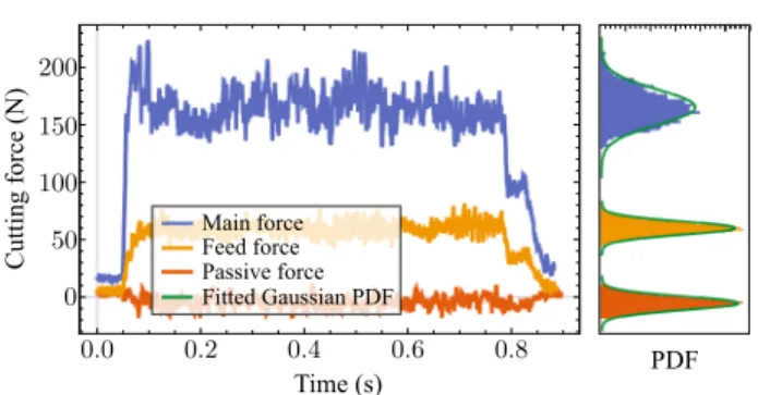
Fig. 1 Examples of force signal components and the corresponding probability density functions (PDFs) measured during a turning operation (the measurement layout is shown in Fig. 3, the cutting velocity isvc=250 mm/min, the rake angle isαc=10◦, and the chip width ish=0.1 mm)
The stochastic differential equations [20] are more efficient tools to approximate these unmodelled dynamic effects. There exists a small number of works employing stochastic differential equations to investigate the effects of fluctuations by modeling them as a white noise excitation.
For example in [21, 22], a mathematical approach with a small number of parameters is presented to describe the magnitude of the noise superposed on the tool motion by means of the stochastic resonance close to the stability boundaries of turning processes. In [23, 24], the cutting process is modeled with the help of stochastic delay differential equations, and the simulated realizations are investigated. Namely, the topological behavior of the high- dimensional point cloud generated from the trajectories is investigated to detect instability near the boundaries of the stable parameter domain. However, the approach, where the fluctuations in the cutting force are modeled as stochastic noise processes, is rarely applied in experimental studies [25]. Usually, these studies are focusing on the slow changes in the cutting force e.g. due to flank wear [26] or heating effects [27].
The novelty of this paper is that it introduces a measurement-based qualitative approach to investigate the high-frequency fluctuations in the cutting force. The resultant effects of these high-speed phenomena are approximated as stochastic Gaussian processes, which has only a small number of parameters, which can be fitted on the measured time signals [28]. This approach leads to stochastic differential equations, which are mathematically complex problems. However, there are many effective, high-performance simulation tools [29–31] to analyze these models. A further advantage of this stochastic description is that it gives a concise description of the fast-varying cutting force by only requiring a small number of parameters.
2 Stochastic cutting force model
The introduced stochastically varying cutting force compo- nentF can be written as:
F (t)=Fm+Fσ(t), (1)
whereFm is the constant mean value of the cutting force and Fσ(t) contains the time-dependent force fluctuation caused by the high-frequency phenomena. These variations are considered the result of large amount and indepen- dent stochastic effects. Therefore, Fσ(t) is a Gaussian- distributed noise since the central limit theorem states that the sum of independent stochastic effects tends to a Gaus- sian normal distributed quantity [20]. Note that F (t) still depends on the cutting parameters, such as chip thicknessh, cutting velocityvc, and rake angleαr:
F (t)=F (t, h, vc, αr, . . .). (2) An efficient way to produce stochastic processes describing Fσ(t) is to use stochastic differential equations, which can be easily simulated with e.g. the Euler-Maruyama method. In this study, two colored noise processes are investigated: first- and second-order filtered Gaussian white noise. The stochastic differential equation of the first-order filter (FOF):
F˙σ+μ1Fσ =σ1Γ (t), (3)
while the second-order filter (SOF) has the form:
F¨σ+2δ2μ2F˙σ +μ22Fσ =σ2μ2Γ (t), (4) whereΓ (t)represents the Gaussian distributed white noise, andμ1,σ1,μ2,σ2, andδ2are the mathematical parameters specific to each parameter set (h, αr, vc). The results of Eqs.3and4are stationary and ergodic processes [20] with stationary deviationsσF:
σF = σ1
√2μ1 = σ2
2√ δ2μ2
, (5)
assuming first- and second-order filters, respectively.
Note that due to the stationarity and ergodicity,σF can be obtained from a single measurement, taking directly the deviation of the measured force signal, independently of which filter is used for modeling the fast-varying partFσ(t) of the cutting force. Furthermore, both processes have zero mean, soFmcontains the average (deterministic) part of the cutting force.
Since the noise intensityσF can be determined without assuming any other property of the cutting force fluctuations Fσ(t), thus a standardized noise process is introduced, namely:
Fσ(t)=σFγ (t). (6)
The noise processγ (t)can be generated with the help of the parametersμ1andμ2,δ2of the original filters in Eqs.3 and 4, respectively. The stochastic differential equations generating the standardized noise processes:
˙
γ (t)+μ1γ (t)=
2μ1Γ (t), (7)
and
¨
γ (t)+2δ2μ2γ (t)˙ +μ22γ (t)=2
δ2μ32Γ (t), (8) for the first- and second-order filters, respectively. Note that in both cases, the process maintains its zero stationary mean E(γ (t)=0); however, its stationary standard deviation is E(γ (t)2)=1.
With this approach, the mean cutting force Fm is calculated as the average of the measured cutting force, and the noise intensity σF is computed with its standard deviation. In order to determine the parameterμ1to fit the the first-order filter, or the parametersμ2andδ2to fit the second-order filter, one has to consider the power spectral density of the process:
γ (t)= F (t)−Fm
σF
. (9)
3 Power spectral density function (PSD)
The power spectrum Sγ(f ) of the standardized cutting force fluctuation γ (t)describes the power distribution in frequency domain. The power spectrum is defined by:
Sγ(f )= lim
T→∞
1
TE(γˆT(f )γˆT∗(f )), (10) where∗denotes the complex conjugate,Eis the expectation value operator,f is the frequency, andγˆT(f )is the bounded Fourier transformation ofγ (t):
ˆ
γT(f )= T 0
e−i2πf tγ (t)dt. (11)
The deterministic functionsSγ(f )can be given in closed forms usingμ1for the first-order filter (12):
Sγ ,1(f )= 2μ1
μ21+(2πf )2, (12)
andμ2,δ2for the second-order filter (13):
Sγ ,2(f )= 4δ2μ32
(μ22−(2πf )2)2+(4π μ2δ2f )2, (13) In practice, the information required to determine the power spectral density of a stochastic process is usually not available; thus, it has to be approximated from a single realization of a process, leading to:
S˜γ(f )= 1
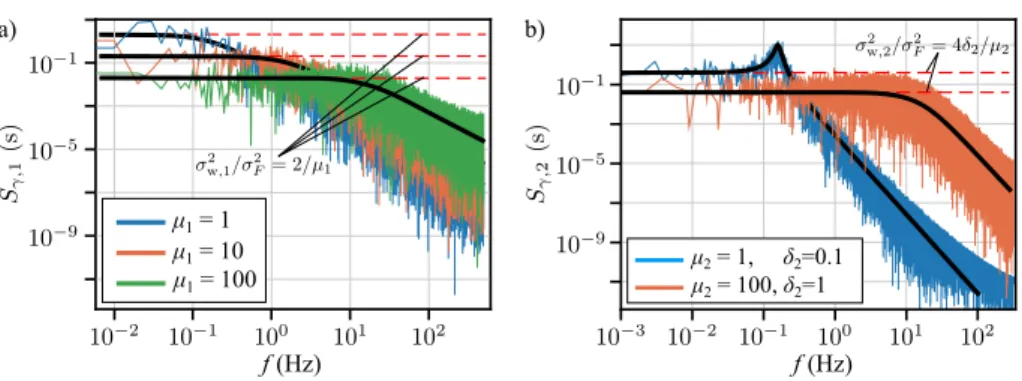
2T(γˆT(f )γˆT∗(f )). (14) Since both the first- and second-order filters are ergodic processes, it is sufficient to fit the power spectrumSγ(f )on the approximationS˜γ(f )of a single measured signal, if the measured time spanT is long enough [32]. The comparison between the analytical power spectral density Sγ(f ) and its approximationS˜γ(f )is demonstrated in Fig.2for both the first- and second-order filters. The realizations used for the power spectral density approximationsS˜γ(f )were computed by numerically integrating the differential (7) for the standardized first-order filter and Eq. 8 for the standardized second-order filter. For the calculations, the Euler-Maruyama method [29] was utilized with time step dt = 10−3 and time spanT = 1000 s, while γˆT(f )was computed using discrete Fourier transformation.
In Fig. 2 it can be observed that the spectral density approximationsS˜γ(f )produce very noisy result; however, they show the main characteristics of their analytical counterpart.
However, if one wants to use the stochastic cutting force for example to see how it affects the stability and stationary behavior of machining processes, the filtered noise approach leads to a nonlinear system. A possible approach to overcome this is to use the white noise process Γ (t)directly to approximate the colored noiseγ (t). Since the white noise has E(Γt1Γt2) = δ(t1 −t2), where δ(.) represents the Dirac-delta, the previously determined noise intensityσF cannot be used for the intensity of the white noiseΓ (t); thus, aσwis introduced. This intensityσwof the white noise processΓ (t)is calculated with the help of the fitted power spectral density functionSγ of the stochastic processγ (t). Since the PSDSγ ,1of the first-order filter does
Fig. 2 Examples of the power spectral densitySγ of the afirst-order filter (12) and bsecond-order filter (13), along with the corresponding approximated power spectral densitiesS˜γ(f )from the single
simulated realizations μ1 = 1
μ1 = 10 μ1 = 100
f (Hz) a)
f (Hz) μ2 = 1, δ2=0.1 μ2= 100, δ2=1 b)
not change significantly up to its cutoff frequencyμ1, the intensityσw is calculated with the help of the maximum of the fitted PSD, which is atω=0, namely:
σw,12 =σF2Sγ(0)= 2σF2 μ1
, (15)
thus leading to σw,1=
√2
√μ1
σF. (16)
For the PSDSγ ,2of the second-order filter a similar white noise intensity approximation is used, leading to:
σw,2=2
δ2
μ2
σF. (17)
4 Measurement
The main goal of the conducted measurements is to show that it is sufficient to use Gaussian stochastic processes to describe the high-frequency fluctuations in the cutting force.
A further goal is to estimate the intensity of the variation of the cutting forceFσ(t)and approximate it as a first- or second-order filters by fitting Sγ ,1(f ) or Sγ ,2(f ) on the power spectra of the measured signals.
The dry orthogonal turning tests were conducted on an NCT EmR-610Ms milling machine, the force signal was measured with a Kistler dynamometer 9129AA and charge amplifier (5080, 5067), and it is registered by National Instruments data acquisition system (NI cDAQ-9178, NI 9234) as shown in the measurement layout in Fig. 3.
The workpieces, AL2024-T351 tubes with 16-mm diameter and 1.5-mm wall thickness, were clamped into the spindle while the carbide tool was fixed on the table. During the experiments, no tool coating or lubricant was used.
The chip thickness h was varied between 0.2 and 0.0005 mm with exponentially decreasing and increasing steps. The orthogonal turning layout allowed realizing the
Fig. 3 Measurement layout
Fig. 4 Example of a raw measured force signal for exponentially decreasing chip thicknesses h with the usually occurring force distributions (blue: accepted as Gaussian, red: not accepted as Gaussian) with parametersvc=250 m/min andαr=5◦
prescribed chip thickness with high precision, even for the small chip thicknesses. This is due to the workpiece having high stiffness in the feed direction, and the chip thickness was controlled by adjusting the feed rate and the spindle speed.
A single force section was measured for around 2 s at a sampling rate 51,200 Hz and there was a 0.1-s pause after every h-step to separate the signal sections while avoiding the cooling of the cutting tool. Due to the fast- varying, stationary, and ergodic characteristic of the cutting force, these measurements were sufficient to determine the parameters of the power spectra of the stochastic cutting force. A typical measured signal with the usually occurring force distributions is shown in Fig.4.
During the measurements, different cutting velocities vc = 50 m/min, 100 m/min, 175 m/min, 250 m/min, and 300 m/min, and rake angles αr = 5◦, 10◦, 15◦, 30◦, 35◦, and 40◦were applied while the relief angle was 10◦for each tool. The tool edge radius was measured using a microscope for each tool, and all of them were found to be smaller than 35 μm. The initial fast wearing of the tools had already taken place before starting the experiments of this work (and measuring the edge radii), and no noticeable tool wear was found during the cutting force measurements.
5 Measurement postprocessing
Due to the measurement setup not only the stochastic variation of the cutting force is obtained. There is a slow change due to the heating of the cutting tool and the workpiece, and a periodic component corresponding to the spindle rotation. The thermal softening effect due to the slowly increasing temperature is visible in Fig.4in the first
∼3 s. This is not related to the piezoelectric dynamometer
Fig. 5 Thermal compensation of the measured cutting force
(Kistler 9129AA) which has a drift in the magnitude of
∼1 N/min which is significantly slower than the cutting force decay we have experienced during the measurements.
Furthermore, the exponential decay almost disappears as the temperature of the cutting reaches its stationary value.
Note that this thermal effect is significant only for the first 4–5 measurement segments (see Fig.4), regardless if the chip thicknesshis increased or decreased between the segments.
To take the thermal effects into account, an exponentially decreasing functionτ (t)is used:
τ (t)=a+bexp(ct), (18)
wherea,b, andc (c < 0)are fitted parameters, using the measured time signalFc,meas(t). The thermal compensated force signal is calculated as follows:
Ftc(t)=Fmeas(t) a
τ (t), (19)
whereFt c(t)denotes the thermal compensated force signal.
Figure5shows the effect of such compensation.
For the next stepFtc(t)is decomposed as:
Ftc(t)=Fm+Fσ,tc(t), (20)
whereFm is the mean and Fσ,tc(t) denotes the variation of the measured and thermal compensated cutting forces.
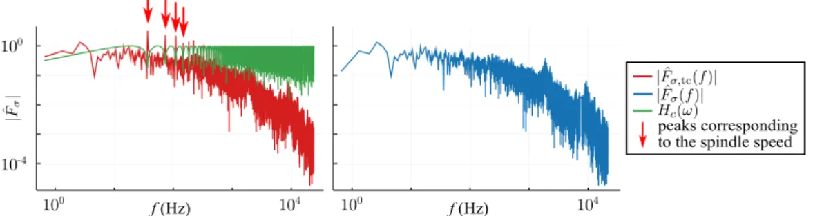
First, the Fourier transformation is applied to the thermal compensated force signalFσ,tc(t), denoted withFˆσ,tc(f ). In
| ˆFσ,tc(f )|, there are peaks at the frequencies corresponding
to the spindle speed and its multiples (see Fig. 6). This originates from the inhomogeneous wall thickness and the eccentricity of the tubes. To eliminate its effect on the power spectra of the measured signal, a filter similar to the so-called comb filter is applied.
Hc(f )= 1 2abs
1−exp
i f
60n
, (21)
wherenis the spindle speed in rpm. Using the product of the Fourier spectrum| ˆFσ,tc(f )|and the comb filterHc(f ),
| ˆFσ(f )|is gained (see Fig.6):
| ˆFσ(f )| = | ˆFσ,tc(f )|Hc(f ). (22) In Eq. 22, | ˆFσ(f )| represents the power spectra of the variation of the measured cutting force originating from the stochastic effects. With the combination of the original phase angle ang
Fˆσ,tc(f ) and the Fourier spectrum of the comb filtered| ˆFσ(f )|the stochastic cutting forceFσ(t)is reconstructed using inverse Fourier transformation. Next, to obtain the standardized cutting force variationγ (t), the intensityσF of the filtered cutting force variationFσ(t)is considered, leading to:
σF =StD
t (Fσ(t)) and γ (t)= Fσ(t) σF
, (23)
where StD
t (Fσ(t)) denotes the standard deviation of the cutting force values obtained during a single measurement step. Now, the power spectra Sγ ,1(f ) and Sγ ,2(f ) of the first and second order filters can be fitted onto the power spectrumSγ(f )of the standardized cutting force variation processγ (t). The fittings were conducted using the package LsqFit.jl [33] in the Julia programming language [34].
Figure 7shows the results of the fitting, namely Fig. 7 a shows the power spectra of the measured post-processed signals, the corresponding fittings Sγ ,1(f ), Sγ ,2(f ), and the fitted white noise intensities σw,1 and σw,2. Panels b and c present example comparisons of the measured and simulated cutting forces F (t) with the first- and second- order filtered noise processes, respectively.
In Fig.7a, it can be observed that the results fitted using the second-order filter show a qualitatively better agreement
Fig. 6 The effect of the comb filter on the power spectrum
Fig. 7 Example comparison of the measured and the fitted cutting force variations with machining parameters h=0.2 mm,vc=100 m/min, andαr=5◦. In panelsaandb, the PSDSγof a measured standardized cutting force variationγ (t )is compared with the fittedSγ ,1with parameter μ1=732 rad/s andSγ ,2with parametersμ2=3022 rad/s, δ2=2.388, respectively, along with the corresponding white noise intensitiesσw,1andσw,2. In panelsbandc, the simulated cutting force is compared with the measurement using first-order filtered noise and second-order filtered noise, respectively
d) c)
FOF SOF
Measurement Fitting
a) b)
than the first-order filter; however, both filters produce similar cutting force patterns compared with the measured force signals.
6 Influence of the machining parameters
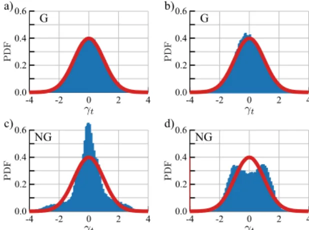
A large number of measurements were conducted with systematically varied cutting parametersh,vc, andαr. Most of the measured signals show a proper Gaussian distribution (Fig. 8, G), for which this stochastic model of the high- frequency phenomena in the cutting force is sufficient.
For chip thicknesses, which are significantly larger than the tool edge radius (h 15μm) and for reasonable cutting velocities (vc > 50m/min), the distribution was Gaussian as noted with green circles in Figs. 9, 10, and 13. However, for smaller chip thicknesses, the distribution deviates notably from the Gaussian (Fig.8, NG); therefore, the proposed stochastic approximation does not hold.
These statistical attributes are denoted by red crosses in Figs. 9, 10, and 13. The force signals were categorized by inspecting the distribution function of each measured signal.
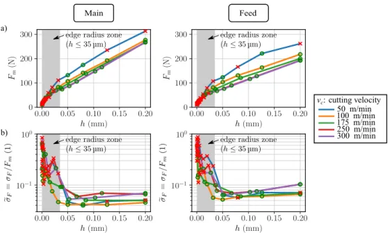
First, the effect of the chip thicknessh on the cutting force is investigated. In Fig.9, it can be observed that the
mean measured cutting force Fm (both the feed and main force components) follows the usual deterministic cutting force characteristics w.r.t. the chip thicknessh[19,35]. In addition, it can be also seen that the intensity of the noise process, relative to the mean, tends to a constant value for chip thicknesses aboveh=0.025–0.1 mm depending on the cutting velocity vc. This means that for conventional chip
0.2 0.4
0.0 0.6
0
-4 -2 2 4
G
0.2 0.4
0.0 0.6
0
-4 -2 2 4
G
0.2 0.4
0.0 0.6
0
-4 -2 2 4
NG
0.2 0.4
0.0 0.6
0
-4 -2 2 4
NG
a) b)
c) d)
Fig. 8 The usually occurring time-distributions of the measured standardized cutting force variations; G, accepted as Gaussian (panels aandb); NG, not accepted as Gaussian (panelscandd)
Feed
50 m/min 100 m/min 175 m/min 250 m/min 300 m/min vc: cutting velocity a)
b)
Main
Fig. 9 aThe average cutting forceFmandbthe intensity of the cutting force fluctuationsFσ(t )with respect to the average value in case of different cutting velocitiesvc(represented with different colors) with
rake angleαr=5◦. In the gray areas the stochastic cutting force model based on the proposed filtered noise processes is not valid, due to the effect of the tool edge radius
thicknesses this noise can be considered a multiplicative noise with intensity:
σF =σFFm, (24)
whereσF denotes the ratio of the deviation and the average of the cutting force. The multiplicative noise intensityσF
takes valuesσF =5–10% if calculated directly from the measured signals andσF = 4–8% if the post-processed signal is investigated, and slightly depends on the cutting parameters, which is analyzed in detail in the Appendix.
This multiplicative nature shows that the noise is present in the cutting force and it is not related to measurement errors.
In case of a small chip thickness h ≤ 35 μm, which is comparable with the cutting edge radius, the multiplicative behaviors of the stochastic variations do not hold anymore (denoted with gray areas in Fig. 9). Furthermore, since in these regions the dominant distribution of the cutting force fluctuations is not Gaussian, the use of the proposed filtered noise processes is not recommended for these chip thicknesses.
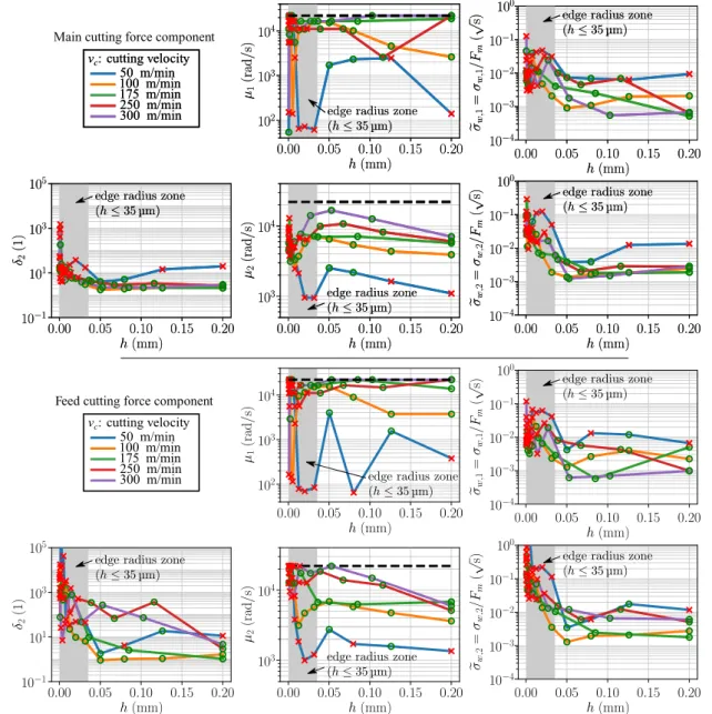
In Fig.10, the results of the power spectra fitting can be seen, namely the behavior of the parametersμ1,μ2, andδ2, along with the white noise intensities σw,1 andσw,2 with respect to the mean cutting forceFm. A general observation is that the parameters of the second-order filterμ2andδ2
show a more regulated tendency with respect to the chip thickness h and cutting velocity vc for all cutting angles αr, compared with the parameter of the first-order filterμ1
(see also theAppendix). Thus, a second-order filtered noise is more appropriate for an accurate mechanical modeling.
Note that for both filtered noise the parametersμ1andμ2
are capped during the fitting process at the natural frequency of the dynamometer denoted with the dashed black lines in Fig.10 atμi =3.5 kHz= 2π×3500 rad/s, i = 1,2 (Fig.11).
Furthermore, similarly to σF, the equivalent white noise intensities σw,1 and σw,2 can also be written as a multiplicative noise with intensity:
σw,1=σw,1Fm and σw,1=σw,2Fm. (25) In case of multiplicative white noise intensity σw,1
computed from the parameter μ1 of the first-order filter, the results show a significant fluctuation with respect to the cutting parameters usually taking values betweenσw,1 = 0.1 and 1%, since μ1 also behaves irregularly. However, the multiplicative white noise intensityσw,2computed from the parametersμ2andδ2of the first-order filter tends to a constant valueσw,2 = 0.1–0.6% with respect to the chip thickness h. The measurement results in Fig. 13 of the Appendix show that the equivalent white noise intensities stay in the interval σw,2 = 0.1–0.6% when varying the cutting velocityvc and the rake angleαr. These intensities are also increased in the case of small chip thicknessesh≤ 35μm, denoted with the gray areas in Figs.10and13, but this effect is not that prevalent as it is for the intensityσF. However, since in these regions the dominant distribution of the cutting force fluctuations is not Gaussian, the model based on the proposed filtered noise processes is not valid anymore.
50 m/min 100 m/min 175 m/min 250 m/min 300 m/min vc: cutting velocity
50 m/min 100 m/min 175 m/min 250 m/min 300 m/min vc: cutting velocity Main cutting force component
Feed cutting force component 50 m/min 100 m/min 175 m/min 250 m/min 300 m/min vc: cutting velocity
Fig. 10 The fitted parameterμ1of the first-order filter, the parame- tersμ2andδ2second-order filter and the relative approximating white noise intensitiesσw,1,σw,2 with respect to the chip thicknesshand cutting velocityvcwith rake angleαr =5◦for the main and the feed
cutting force components. The dashed line denotes the constraintμi≤ 3.5 kHz,i=1,2. In the gray areas, the stochastic cutting force model based on the proposed filtered noise processes is not valid, due to the effect of the tool edge radius
7 The effect on the dynamics of machining
To demonstrate the effect of the stochastic cutting force on the dynamics of cutting processes [15], the simple one degree of freedom regenerative model of turning is used [1, 36]:
¨
z(t)+2ζ ωnz(t)˙ +ωn2z(t)= 1
mF (t). (26)
In this model, the cutting tool is considered a linear oscillator with natural frequencyωn=√
k/mand damping coefficientζ =c/m, wherem,k, andcare the modal mass, stiffness, and the viscous damping, respectively.
This oscillator is excited by the stochastic cutting force F (t)depending on the chip thicknessh, which is described by the regenerative effect, calculated using the actual and delayed tool positions [37]:
h(t)=h0+z(t−τ )+z(t). (27)
The delayτ corresponds to the the spindle speedof the workpiece, namelyτ =/2π.
To analyze the small amplitude vibration around the stationary position, the widely used deterministic shifted linear cutting force model is considered [1,3,7,36,38] for
Fig. 11 Mechanical model of turning
the meanFm: Fm(h(t))=Kz
h∗+h(t)
, (28)
whereKz is the resultant cutting force coefficient, which includes the average effects of the material properties as well as the chip widthw, whileh∗is the shift parameter.
To simulate the turning process using the proposed first- or second-order filtered colored noise processes, one has to fit the parametersμ1(h)orμ2(h)and δ2(h) according to Fig. 10. After this fitting, one can use Eqs. 1, 3, 26, and 27 to simulate the vibrations of the tool during the turning operation. However, applying any of the colored noises defined in Eqs.3or4leads to nonlinear stochastic delay differential equations.
Fortunately, in most practical cases, the dominant natural frequencies are less than 1 kHz, while the parametersμ1/2π andμ2/2π are in the range of 2–3 kHz (ωn μi, i = 1,2). Thus, in the frequency range of the dominant natural frequencies, the power spectra Sγ ,1 and Sγ ,2 of the FOF and SOF are approximately constant, while the higher
frequencies are already filtered out by the mechanical system. This property can be utilized by applying the stochastic force model with the equivalent Gaussian white noise processΓ (t)with the multiplicative noise intensity as described in Eq.24, leading to:
Fσ(t)=σwFm(h(t))Γ (t). (29) This approach leads to linear stochastic delay differential equations, and allows the computation of stability and stationary behavior. With these assumptions, the stochastic cutting force is described as:
F (t)=Kz
h∗+h(t)
(1+σwΓ (t)). (30) Substituting (27) and (30) into Eq.26leads to:
¨
z(t)+2ζ ωnz(t)˙ +ω2nz(t)
=H (h∗+h0+z(t−τ )−z(t)) +σwH (h∗+h0+z(t−τ )−z(t))Γ (t),
(31)
where H = Kz/m. To investigate the stochastic pertur- bation of the mean stationary solution E(zst), a stochastic perturbation processy(t)is introduced:
z(t)=E(zst)+(h∗+h0) y(t), (32) where
E(zst)=(H /ω2n)(h∗+h0). (33) Note thaty(t)has zero meanE(y(t))=0. Thisy(t)process describes the motion of the tool around its equilibrium position and is normalized with the shifted-nominal chip thickness. Substituting (32) into (31) leads to:
doty(t)+2ζ ωny(t)˙ +ωn2y(t)
=H (y(t −τ )−y(t))
+σwH (1+y(t−τ )−y(t))Γ (t).
(34)
Fig. 12 aSecond moment stability chart (blue area) along with stationary second moment limiting charts (darker blue areas) with parameterσw=1%, compared with the deterministic stability borders.bNoise magnification in the stationary solution alongκ=0.3. There are three small figures inside illustrating how the first moment decays (dark blue) while the stochastic vibrations persist (light blue) for different spindle speeds
a)
10 50 40 30 20
0.4 0.6 0.8 1.0 1.2 1.4 1.6
b)
15x noise ampli fication 30x noise ampli fication 15x noise amplificat ion Second moment stable area
0.6 .8 1.0 1.2 1.4 1.6
0.4
30x noise amplificat ion Deterministic model's stability border
0
This perturbation equation can be rewritten into the usual representation of a stochastic differential equation, the first- order incremental form [20,32]:
dx(t)= (Ax(t)+Bx(t−τ ))dt
+(αx(t)+βx(t−τ )+σ)dW (t), (35) where
x(t)= y(t)
˙ y(t)
,A=
0 1
−
ωn2+H
−2ζ ωn
,B=
0 0 H 0
, α=
0 0
−σwH 0
, β=
0 0 σwH 0
, σ =
0 σwH
. (36) The increment dW (t) represents the Wiener increment, originating from the integration of the white noise process Γ (t), namely:
dW (t)=W (t+dt)−W (t):= t+dt t
Γ (s)ds. (37) If the equation system is in the form shown in Eq.35, the stationary mean and variance of the process and their sta- bility can be calculated by supplying the coefficient matri- ces (36) to the packageStochasticSemiDiscretization.jl[39]
written in Julia. This package is based on the stochastic semidiscretization [31] of linear stochastic delay differential equations.
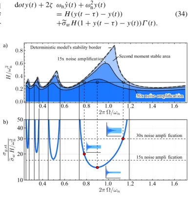
In Fig. 12 a, the stability chart is shown, where the unstable and stable areas are denoted with white and blue colors, respectively. The calculations were conducted using the damping ζ = 0.1 and as an overestimation of the stochastic effectsσw = 0.01 (which corresponds to a 1%
multiplicative white noise intensity compared with the mean cutting force). To see the effect of the noise originating from the cutting force, the stability boundary for the deterministic case is plotted with dashed lines based on the analytical solution presented in [37].
When comparing the stability boundaries gained with the stochastic and deterministic models, it can be observed that the change in stability is insignificant; the deterministic model is sufficient for the stability calculations. However, if one considers the stationary vibrations caused by the small stochastic cutting force, the noise intensity in the vibrations can be amplified. This can dramatically increase the surface roughness since this vibration is directly copied onto the surface, and it can lead to additional loads on the tool.
To characterize the intensity of these stochastic vibra- tions, the stationary standard deviation of the displacement perturbationy(t)is used, namely:
σy,st:= lim
t→∞
E(y(t)2). (38)
By defining a limit (e.g., based on a prescribed surface quality requirement), the stationary second moment chart can be given by the contour lines of Eq.38. In Fig.12a,
two contours are given for 15 and 30 times dimensionless noise amplification, namely σy,st/(σwH ω2n) = 15 and 30.
The darker blue areas correspond to the parameter regions, where the noise amplification is limited by these values.
Although the stability limit (both the deterministic and stochastic) provides stability pockets with optimal high material removal rates, these optimums cannot be utilized due to the large stationary stochastic vibrations.
In Fig. 12 b, the stationary second moment due to the noise induced resonance is illustrated along the parameter lineH /ω2n=0.3. These vibrations are extremely amplified near the stability borders; this phenomenon is due to the noise-induced stochastic resonance [40]. Note that these theoretical predictions are only valid for small amplitude vibrations due to the nonlinear nature of the cutting force characteristics [38] and the fly-over effect [41].
If in the stable parameter region the vibrations reach a sufficiently large stationary second moment (and therefore large amplitudes), the chatter vibration can occur before the machining would lose the stability predicted with the help of deterministic linear models. This means that the measurable stability boundaries are potentially shifted toward smaller chip widths by the stochastic excitation from the cutting force. In Fig.12b, it can be seen that as the spindle speed is chosen from the immediate proximity of the stability boundary the effect of the stochastic noise is significantly magnified even though the intensity of the noise stays constant. This phenomenon can be due to the fact that the white noise excites through the whole frequency spectrum, and the characteristic damping of the dynamical system representing the turning process decreases, reaching zero at the stability boundary. This means, that even if the presence of the additive stochastic effect is small, it can cause significant vibrations due to the stochastic resonance, despite the system being asymptotically stable.
8 Summary and discussion
In this work, it is showed, through extensive measurements, that the cutting force is an inherently stochastic process, and the noise during the tests originates from the cutting process, and it is not related to the measurement error.
First, a mathematical description of the stochastic behavior of the cutting force is given, then the spectral properties of the proposed first- and second-order filter are described in an analytical form. A systematic series of orthogonal turning tests were conducted to identify the parameters of these models. Before the parameters of the proposed noise processes were fitted, the thermal effect and the periodic component related to the spindle rotation, a post-process is performed using exponential compensation and comb filter. The first- and second-order filters could be
Fig. 13 The effect of the rake angle αr and the cutting velocityvc
on the average cutting forceFm, the relative cutting force fluctuation σF, the parameterμ1of the first-order filtered noise, the parameters
μ2and δ2 of the second-order filtered noise, and the relative white noise intensitiesσw,1andσw,1 for the main and feed cutting force components
fitted well on the post-processed measured signals; however, the second-order filter produced more regular results, with respect to the machining parameters.
The second-order filter was able to produce the slope that can be observed in the power spectral density of the measured cutting force (see Fig. 7), and it has two parameters,μ2andδ2. Due to the frequency response of the Kistler dynamometer 9129AA, the measured power spectral density function was valid only up to 3.5 kHz; thus, the parameterμ2was limited during the fitting, namelyμ2 ≤ 2π×3500 rad/s. Furthermore, the largeδ2values (δ2≥10) suppress the peak usually observable in the power spectrum of a second-order system. Thus, the flat characteristic of the power spectrum of the first-order filter is retained, with the increased steepness specific to the power spectrum of the second-order filter.
Note that the fitting of the parameters of the proposed noise processes is still challenging, and during our measurements we did not find as clear patterns in the behavior of μ1 μ2, δ2, σw,1 and σw,2 with respect to the machining parameters as in case of the mean cutting force. However, compared with a FEM model, the filtered noise processes (7) and Eq. 8 require only one or two parameters, providing magnitudes of order more with a concise description than FEM models, with only one or two parameters.
Furthermore, it is shown in Fig.7 c and d that, using the fitted parameters and the corresponding stochastic differential (3) and (4), an approximating realization of the stochastic force signal can be generated. Since the stochastic noise processes used in this study can be generated with small computation resources, and there are even well- established tools such as the Differentialequations.jlJulia package [30] that can integrate small stochastic differential equations with high performance, thus this approach is order of magnitudes faster compared with detailed finite element models.
During the detailed analysis of the effect of the machining parameters, namely the chip thickness h, the cutting velocityvc, and the rake angleαr, it is found that the stochastic component can be considered multiplicative noise outside the edge radius zone, namely for uncut chip thicknesses h > 35 μm. The parameters μ2 and δ2
of the second-order filtered noise show more consistent dependency on the technological parameters, than the parameter of the first-order filtered noise; thus, a SOF noise is recommended to be used during simulations. The intensity of the cutting force noise was aroundσF =4 %− 8 % of the mean, and the parameterμ2/(2π )is in the range of 2−3 kHz, while the parameter δ2 has a magnitude of δ2∝10.
To further simplify the noise model, the use of the white noise process Γ (t) is recommended to model the
stochastic component of the cutting force. In this work, the power spectral density function of a filtered noise process is approximated with the constant power spectrum of the Gaussian white noise. The intensity σw of the white noise process is calculated from the parameters of the filtered noise processes according to Eqs. 16 and 17.
The measurements show that the equivalent white noise excitation has an intensity of σw = 0.1–1% of the mean. Since the parametersμ2 andδ2 of the second-order filter show the more regular behavior with respect to the technological parameters, a similar characteristic can be observed for the white noise intensityσw,2calculated from these parameters.
For the qualitative analysis of a turning process, choos- ing a relative white noise intensityσw =0.1–1% is a safe choice. However, when modeling the fluctuations in the cutting force using one of the filtered noises, it is recom- mended to conduct the measurements for the investigated tool, workpiece, and machining layout. The parameters of the filtered noises influence the characteristics of the simu- lated cutting force significantly, since not only the intensity of the fluctuations is considered, but also the frequencies at which the power is supplied to the mechanical sys- tem describing the machine tool. In contrast, in case of a white noise approximation, even the concept itself is an approximation, since there is no physical process supplying constant power on all the frequencies. Thus, using a white noise to model the fluctuations in the cutting force is a rough estimation even with a measured intensityσw; hence, it is sufficient to considerσw of magnitudeσw ∝ 10−3−10−2 without measurements.
In the final section, to demonstrate the significance of the stochastic description of the cutting force, a simple model of the orthogonal turning was investigated. It was shown how the noise in the cutting force influences the behavior of the turning process and how even a seemingly negligible stochastic excitation can lead to stochastic coherence resonance which always occurs near the stability boundaries. This resonance caused by the stochastic excitation from the cutting force can be a potential explanation to the measurement difficulties of theoretically predicted stability charts [42, 43]. Furthermore, these stationary vibrations can cause the transition to chatter in the multistable zones near the stability borders [6,44].
9 Conclusion
It is shown that the cutting force is a stochastic process, and the following properties should be considered:
– An overall relative noise intensity ofσF = 4–8% was measured depending on the parameters of the turning.
– Stochastic processes described by models with small number of parameters can be fitted on the fluctuations of the cutting force.
– From the two fitted stochastic processes, the second- order filtered noise showed more regular and better fit, than the first-order filtered noise.
– A Gaussian white noise estimation is also given with intensityσw =0.1–0.6% of the mean cutting forceFm. – This small amount of noise in the cutting force does not influence the stability properties of the milling process, but the stationary vibrations due to the noise- induced resonance. These stationary vibrations can cause unacceptable surface quality, makes it harder to detect chatter, or it can even cause a transition to chatter in multistable zones near the stability borders.
Funding Open access funding provided by Budapest University of Technology and Economics. This work was funded by the Hungarian Ministry of Human Capacities (NTP-NFT ¨O-19-B-0127) and supported by the Hungarian Scientific Research Fund (OTKA FK- 124462, PD-124646) and by the National Research, Development and Innovation Fund (TUDFO/51757/ 2019-ITM, Thematic Excellence Program).
Open Access This article is licensed under a Creative Commons Attribution 4.0 International License, which permits use, sharing, adaptation, distribution and reproduction in any medium or format, as long as you give appropriate credit to the original author(s) and the source, provide a link to the Creative Commons licence, and indicate if changes were made. The images or other third party material in this article are included in the article’s Creative Commons licence, unless indicated otherwise in a credit line to the material. If material is not included in the article’s Creative Commons licence and your intended use is not permitted by statutory regulation or exceeds the permitted use, you will need to obtain permission directly from the copyright holder. To view a copy of this licence, visit http://
creativecommonshorg/licenses/by/4.0/.
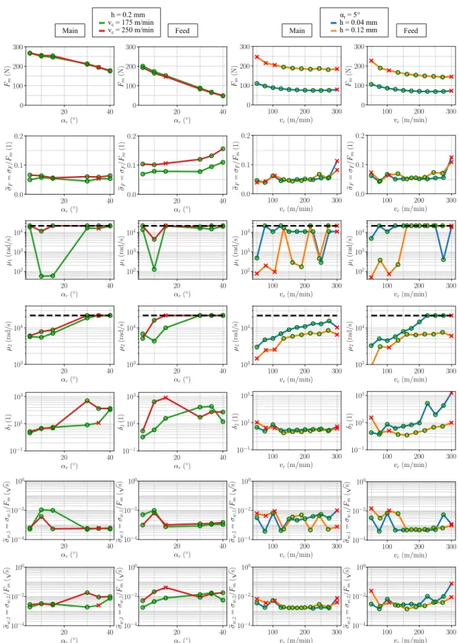
Appendix
Figure13shows the influence of the machining parameters rake angle αr and the cutting velocity vc on the average cutting force Fm, the relative intensity σF of the cutting force fluctuation, the parameterμ1of the first-order filtered noise, the parametersμ2andδ2of the second-order filtered noise, and the relative white noise intensitiesσw,1andσw,1
for the main and feed cutting force components. The main and the feed components of the mean cutting forceFmhave a similar decreasing tendency for increasing cutting angle αr as in [35], while the velocity dependency shows the usual power function characteristic with a small negative exponent. The relative noise intensityσF changes slightly as a function of these parameters; however, the independence ofσF from rake angleαrand the cutting velocityvccannot be concluded due to the small number of measurements. The more regulated behavior with respect to the rake angleαr
and the cutting velocityvcof the parameters of the second- order filtered noise can also be observed, similarly as in Fig.10. Here, the parametersμ1andμ2are again restricted by the natural frequency of the dynamometer, denoted with the dashed lines in the corresponding diagrams. The approximating relative white noise intensities are also in the range ofσw =0.1–1%; furthermore,σw,2shows especially small sensitivity to the technological parametervc.
References
1. Tobias S (1965) Machine-tool vibration. Blackie, Glasgow 2. Insperger T, Mann BP, St´ep´an G, Bayly PV (2003) Stability of up-
milling and down-milling, part 1: alternative analytical methods.
Int J Mach Tools Manuf 43(1):25–34. https://doi.org/10.1016/
s0890-6955(02)00159-1
3. Insperger T, Stepan G, Bayly PV, Mann BP (2003) Multiple chatter frequencies in milling processes. J Sound Vib 262(2):333–
345.https://doi.org/10.1016/S0022-460X(02)01131-8
4. Mann BP, Insperger T, Bayly PV, St´ep´an G (2003) Stability of up-milling and down-milling, part 2: experimental verification. Int J Mach Tools Manuf 43(1):35–40.https://doi.org/10.1016/s0890- 6955(02)00160-8
5. Tamas I (2010) Full-discretization and semi-discretization for milling stability prediction: Some comments. Int J Mach Tool Manuf 50:658–662. https://doi.org/10.1016/j.ijmachtools.2010.
03.010
6. Dombovari Z, Iglesias A, Molnar TG, Habib G, Munoa J, Kuske R, St´ep´an G (2019) Experimental observations on unsafe zones in milling processes. Philos Trans R Soc A 377:2153.
https://doi.org/10.1098/rsta.2018.0125
7. Insperger T, Mann BP, Surmann T, Stepan G (2008) On the chatter frequencies of milling processes with runout. Int J Mach Tools Manuf 48(10):1081–1089. https://doi.org/10.1016/j.ijmachtools.
2008.02.002
8. Gyebr´oszki G, Bachrathy D, Csern´ak G, St´ep´an G (2018) Stability of turning processes for periodic chip formation. Adv Manuf 6(3):345–353.https://doi.org/10.1007/s40436-018-0229-6 9. Palmai Z, Csernak G (2009) Chip formation as an oscillator during
the turning process. J Sound Vib 326:809–820.https://doi.org/10.
1016/j.jsv.2009.05.028
10. Prohaszka J, Dobranszky J (2003) The role of an anisotropy of the elastic moduli in the determination of the elastic limit value. Mater Sci Forum 414-415:311–316.https://doi.org/10.4028/www.scien tific.net/MSF.414-415.311
11. Prohaszka J, Dobranszky J, Nyir´o J, Horvath M, Mamalis A (2004) Modifications of surface integrity during the cutting of copper. Mater Manuf Process 19:1025–1039.https://doi.org/10.
1081/AMP-200035192
12. Prohaszka J, Mamalis AG, Horvath M, Nyiro J, Dobranszky J (2006) Effect of microstructure on the mirror-like surface quality of fcc and bcc metals. Mater Manuf Process 21(8):810–818.
https://doi.org/10.1080/10426910600837806
13. Berezvai S, Molnar T, Bachrathy D, Stepan G (2018) Experimen- tal investigation of the shear angle variation during orthogonal cut- ting. Mater Today: Proc 5:26495–26500.https://doi.org/10.1016/
j.matpr.2018.08.105
14. Munoa J, Beudaert X, Dombovari Z, Altintas Y, Budak E, Brecher C, Stepan G (2016) Chatter suppression techniques in metal cutting. CIRP Ann Manuf Technol 65(2):785–808.https://doi.org/
10.1016/j.cirp.2016.06.004
15. Sykora H, Bachrathy D, St´ep´an G (2017) A theoretical investigation of the effect of the stochasticity in the material properties on the chatter detection during turning. In: 29th Conference on Mechanical Vibration and Noise, vol 8. American Society of Mechanical Engineers (ASME)
16. Berezvai S, Molnar TG, Kossa A, Bachrathy D, Stepan G (2019) Numerical and experimental investigation of contact length during orthogonal cutting. Mater Today: Proc 12:329–334.
https://doi.org/10.1016/j.matpr.2019.03.131
17. Chełminski K, H¨omberg D, Rott O (2011) On a thermomechanical milling model. Nonlinear Anal Real World Appl 12(1):615–632.
https://doi.org/10.1016/j.nonrwa.2010.07.005
18. Wojciechowski S, Matuszak M, Powałka B, Madajewski M, Maruda RW, Kr´olczyk GM (2019) Prediction of cutting forces during micro end milling considering chip thickness accumula- tion. Int J Mach Tools Manuf 147:103466.https://doi.org/10.1016/
j.ijmachtools.2019.103466
19. Altintas A, Ber R (2001) Manufacturing automation: Metal cutting mechanics, machine tool vibrations, and cnc design. Appl Mech Rev 54(5):B84–B84.https://doi.org/10.1115/1.1399383
20. Oksendal B (2003) Stochastic differential equations. Springer, Berlin
21. Buckwar E, Kuske R, L’esperance B, Soo T (2006) Noise- sensitivity in machine tool vibrations. Int J Bifur Chaos 16(08):2407–2416
22. Kuske R (2010) Competition of noise sources in systems with delay: the role of multiple time scales. J Vib Control 16(7-8):983–
1003.https://doi.org/10.1177/1077546309341104
23. Khasawneh FA, Munch E (2016) Chatter detection in turning using persistent homology. Mech Syst Signal Process 70-71:527–
541.https://doi.org/10.1016/j.ymssp.2015.09.046
24. Khasawneh FA, Munch E (2017) Utilizing topological data analysis for studying signals of time-delay systems. In: Insperger T, Ersal T, Orosz G (eds) Time delay systems: theory, numerics, applications, and experiments. Springer, Cham, pp 93–106 25. Nieslony P, Krolczyk GM, Wojciechowski S, Chudy R, Zak K,
Maruda RW (2018) Surface quality and topographic inspection of variable compliance part after precise turning. Appl Surf Sci 434:91–101.https://doi.org/10.1016/j.apsusc.2017.10.158 26. Patel VD, Gandhi AH (2019) Modeling of cutting forces
considering progressive flank wear in finish turning of hardened AISI d2 steel with CBN tool. Int J Adv Manuf Technol 104(1- 4):503–516.https://doi.org/10.1007/s00170-019-03953-2 27. Farahnakian M, Elhami S, Daneshpajooh H, Razfar MR (2016)
Mechanistic modeling of cutting forces and tool flank wear in the thermally enhanced turning of hardened steel. Int J Adv Manuf Technol 88(9-12):2969–2983. https://doi.org/10.1007/s00170- 016-9004-7
28. Sykora HT, Bachrathy D, Stepan G (2018) Gaussian noise process as cutting force model for turning. Procedia CIRP
77:94–97.https://doi.org/10.1016/j.procir.2018.08.229. 8th CIRP Conference on High Performance Cutting (HPC 2018)
29. Kloeden PE, Platen E, Schurz H (2012) Numerical solution of sde through computer experiments. Springer, Berlin
30. Rackauckas C, Nie Q (2017) Differentialequations.jl – a perfor- mant and feature-rich ecosystem for solving differential equations in julia. J Open Res Softw 5.https://doi.org/10.5334/jors.151 31. Sykora HT, Bachrathy D, Stepan G (2019) Stochastic semi-
discretization for linear stochastic delay differential equations. Int J Numer Methods Eng 119(9):879–898.https://doi.org/10.1002/
nme.6076
32. Arnold L (1973) Stochastic differential equations: theory and applications. R. Oldenbourg Verlag, Munich
33. White JM Julia package: Lsqfit.jl, v0.3.3. https://github.com/
JuliaNLSolvers/LsqFit.jl
34. Bezanson J, Edelman A, Karpinski S, Shah VB (2017) Julia: a fresh approach to numerical computing. SIAM Rev 59(1):65–98.
https://doi.org/10.1137/141000671
35. Molnar TG, Berezvai S, Kiss AK, Bachrathy D, Stepan G (2019) Experimental investigation of dynamic chip formation in orthogonal cutting. Int J Mach Tools Manuf 145:103429 36. Tlusty J, Spacek L (1954) Self-excited vibrations on machine
tools. Nakl. CSAV, Prague, Czech Republic
37. Stepan G (1989) Retarded dynamical systems: stability and characteristic functions, research notes in mathematics series, vol 210. Wiley, New York
38. Altintas Y (2011) Manufacturing Automation. Cambridge Univer- sity Press, Cambridge
39. Sykora HT (2019) Julia package: Stochasticsemidis- cretizationmethod.jl, v0.3.3. https://github.com/HTSykora/
StochasticSemiDiscretizationMethod.jl
40. Kuske R (2006) Multiple-scales approximation of a coher- ence resonance route to chatter. Comput Sci Eng 8(3):35–43.
https://doi.org/10.1109/MCSE.2006.44
41. Dombovari Z, Barton DAW, Eddie Wilson R, Stepan G (2011) On the global dynamics of chatter in the orthogonal cuttingmodel.
Int J Non-Linear Mech 46(1):330–338.https://doi.org/10.1016/j.
ijnonlinmec.2010.09.016
42. Schmitz TL (2003) Chatter recognition by a statistical evaluation of the synchronously sampled audio signal [2]. J Sound Vib 262(3):721–730.https://doi.org/10.1016/S0022-460X(03)00119-6 43. Altintas Y, Chan PK (1992) In-process detection and suppression
of chatter in milling. Int J Mach Tools Manuf 32(3):329–347.
https://doi.org/10.1016/0890-6955(92)90006-3
44. Moln´ar TG, Insperger T, Hogan SJ, St´ep´an G (2016) Estimation of the bistable zone for machining operations for the case of a distributed cutting-force model. J Comput Nonlinear Dyn 11(5) Publisher’s note Springer Nature remains neutral with regard to jurisdictional claims in published maps and institutional affiliations.