The Short-Term Effects of Experimental Forestry Treatments on Site Conditions in an Oak–Hornbeam Forest
Bence Kovács1,2,3,*ID, Flóra Tinya1, Erika Guba1, Csaba Németh2, Vivien Sass4, András Bidló4 and PéterÓdor1,2 ID
1 MTA Centre for Ecological Research, Institute of Ecology and Botany, Alkotmányút 2-4, H-2163 Vácrátót, Hungary; tinya.flora@okologia.mta.hu (F.T.); csillagfonal@gmail.com (E.G.);
odor.peter@okologia.mta.hu (P.Ó.)
2 MTA Centre for Ecological Research, GINOP Sustainable Ecosystems Research Group, Klebelsberg Kuno utca 3, H-8237 Tihany, Hungary; nemeth.csaba@okologia.mta.hu
3 Department of Plant Systematics, Ecology and Theoretical Biology, Eötvös Loránd University, Pázmány Péter Sétány 1/C, H-1117 Budapest, Hungary
4 Institute of Environmental and Earth Sciences, University of Sopron, Bajcsy-Zsilinszky utca 4, H-9400 Sopron, Hungary; sass.vivien@uni-sopron.hu (V.S.); bidlo.andras@uni-sopron.hu (A.B.)
* Correspondence: kovacs.bence@okologia.mta.hu; Tel.: +36-28-360-122 (ext. 107)
Received: 4 June 2018; Accepted: 3 July 2018; Published: 5 July 2018
Abstract:Forest management alters forest site; however, information is still limited about how different silvicultural treatments modify abiotic conditions. We compared the effects of four treatments from three different forestry systems on forest microclimate, litter, and soil conditions. The clear-cutting, retention tree group, preparation cutting, and gap-cutting treatments were experimentally established in a European oak-dominated forest, following a complete block design with six replicates. In this study, we show the results of the quantitative analyses of 21 variables, one year after the interventions.
Strong treatment effects were observed for the microclimate and litter variables, whereas the soil characteristics remained similar. The increase in light was the highest in the clear-cuts with intermediate effects in the gap-cuts. The means and variances of the air and soil temperature as well as the vapor pressure deficit were the highest for the clear-cutting treatment. An increase in soil moisture, litter pH, and litter moisture was significant in the gap-cuts and, to a smaller extent, in the clear-cuts. The soil pH increased in the retention tree groups. Microclimatic differences between the treatments were the largest during the summer, which demonstrates the buffering effect of the canopy. Our study confirms that less intensive and more spatially heterogeneous silvicultural treatments (e.g., gap-cutting) preserve a stable below-canopy microclimate more effectively. These results can support and might be useful for both forest management and conservation planning.
Keywords:forest site conditions; microclimate; soil; litter; temperate deciduous forest; field experiment;
forest management
1. Introduction
Forest management induces substantial alterations in environmental conditions that fundamentally influence the ecosystem’s structure and functions [1,2]. These strongly impact the long-term survival, regeneration, and diversity of forest-dwelling organism groups [3,4].
Silvicultural treatments can directly generate changes in forest biodiversity by deteriorating communities associated with individual trees and tree-related microhabitats, such as epiphytes [5], deadwood-dependent communities [6], and cavity nesters [7]. Most of the forest-dependent taxa are
Forests2018,9, 406; doi:10.3390/f9070406 www.mdpi.com/journal/forests
Forests2018,9, 406 2 of 23
indirectly influenced by forest management through the alteration of site conditions—microclimate, litter attributes, and soil characteristics—and biogeochemical cycles [8–12]. The microclimate is also a major driver of ecosystem processes such as decomposition, respiration, and nutrient dynamics [13,14]. Studying the effects of different management practices on forest site conditions can support the mitigation of the negative impacts of climate change [15,16], because fine-scale measurements and high-resolution models are necessary to create predictions for the ecological processes or calculate probable species distributions [17,18]. Therefore, for conservation purposes, it is important to investigate how forestry treatments alter forest site conditions through numerous, highly interrelated effects.
Forest stands create a unique, buffered below-canopy microclimate [19,20] compared to open-fields [21] or to plantations [22]. This buffering capacity is mainly determined by the tree species composition, tree species richness, and stand structure, as the foliage of the different vegetation layers absorbs a large proportion of incoming solar energy and reduces the loss of longwave radiation from the surface [21,23–25]. The soil and litter characteristics are also influential [26,27]. As a result of these effects, forest microclimates can be characterized by lower diurnal and seasonal magnitudes, in case of several microclimatic variables [19,26]. Similarly, the litter layer is important for many decomposer groups as a habitat and food resource, as well as for nutrient cycling, smoothing the fluctuations of the physical and chemical properties of the topsoil, and the below-canopy ambient air [9,28].
Alterations of the microclimate, litter, and soil properties, and thus changes in forest communities, are highly dependent on the spatial extent, the spatiotemporal pattern, frequency, and severity of the forest management approaches applied [29–31]. Changes in the main structural elements of forests (e.g., canopy closure, horizontal, and vertical foliage distribution) result in considerable alterations in the processes of the soil–vegetation–atmosphere system. This effect is obvious for clear-cuts [32–34], but it is also observable in partial cuts like thinning, group selection, or retention tree harvesting [11,35–39].
Even though forest management in the temperate zone is shifting globally from even-aged rotation management systems towards continuous-cover silvicultural approaches that support structural heterogeneity, we have limited information about how the different forestry interventions affect the forest site conditions [31]. Forestry experiments are necessary for the understanding of the complex relationships between different management practices and forest site, regeneration, and biodiversity characteristics.
However, as Bernes et al. pointed out, there is a knowledge gap concerning the possible multipurpose forest management alternatives in Central European deciduous forests [40]. There are studies that examine the effects of multiple treatment levels within a particular silvicultural system on microclimate, such as different artificial gap sizes and shapes [35,41], various combinations of retention levels and spatial configurations [36], thinning intensities and patterns [42,43], and fuel-reduction oriented treatments [44].
Similarly, changes in soil characteristics and biochemical processes have been shown in lower intensity harvest types [13,37,39,45]. Most of the studies dealing with the interactions between harvesting and forest site conditions concentrate on one selected forestry system. Two or more silvicultural strategies have rarely been applied within one experimental design (but see, for example, [11] or [14]).
The ‘Pilis Experiment’ was implemented to compare the effects of different treatment types on site conditions, regeneration and biodiversity. All of the alternative silvicultural systems applicable to European forests were included (clear-cutting, shelterwood system and continuous-cover forestry with gap-cutting; [46]). All of the established treatment types—clear-cutting, gap-cutting, preparation cutting, and retention tree group—are common practice in the temperate regions of Europe. To model large clear-felled areas (usually created by the clear-cutting system or shelterwood system, in the course of the final cutting), clear-cutting was applied. This is the most extreme yet widespread silvicultural treatment type, applied in even-aged rotation forestry. The study of retention tree groups inside clear-cuts is particularly interesting. Recently, the application retained groups of individuals has been spreading, as they mitigate the impacts of clear-cutting, an important goal of nature conservation in forests. The shelterwood system is represented here in the form of preparation cutting, which is the first step towards the final cutting. Moreover, it is a form of partial cutting, comparable to thinning or dispersed green tree retention. In Central Europe, continuous cover forestry is typically practiced
via artificial gaps or group selection, therefore, gap-cutting was also part of our study. Our open-field, multi-taxa experiment was established in 2014 [47]. As a target habitat type, sessile oak (Quercus petraea Matt. [Liebl.]) and hornbeam (Carpinus betulusL.) forests were chosen, which represent a deciduous woodland habitat type widespread in the Pannon Ecoregion [48] and generally in Central Europe [49].
This is one of the focal indigenous forest types for timber harvesting in this region, because of the high-quality timber of sessile oak [50]. Here, we focus on the effects of the experimental treatments on site conditions during the first post-harvest period. Our objectives are to quantify the differences induced by the applied management treatments (clear-cutting, gap-cutting, preparation cutting, and retention tree group) (1) on the mean and variability of microclimate, soil, and litter variables during the growing season; (2) on the temporal pattern of site condition variables through a growing season; and (3) on the diurnal patterns of selected microclimate variables.
We hypothesized that the microclimate responds to the treatments immediately, whereas changes in the litter and soil variables were expected to be delayed. Clear-cutting affects the forest site most strongly. For the majority of our variables, we supposed that the retention tree group mitigates the harsh environmental conditions generated by clear-cutting. We presumed that gap-cutting and preparation cutting cause intermediate changes in the forest site conditions. We also presumed that differences from the control are more expressed in the summer, at the peak of the growing season, when the canopy closure of the control is the highest. This will also be discernible in the form of larger disjunctions in the diurnal cycles of the microclimate.
2. Materials and Methods
2.1. Study Area
The study was conducted in the Pilis Mountains, north-eastern ridge of the Transdanubian Range, Hungary (47◦400 N, 18◦540 E; Figure1a). Plots are situated on a horst ridge (370–470 m above sea level) on moderate (7.0–10.6◦), north-facing slopes. The average annual mean temperature is 9.0–9.5◦C (16.0–17.0◦C during the growing season), with a mean annual precipitation of 650 mm [51].
cutting, which is the first step towards the final cutting. Moreover, it is a form of partial cutting, comparable to thinning or dispersed green tree retention. In Central Europe, continuous cover forestry is typically practiced via artificial gaps or group selection, therefore, gap-cutting was also part of our study. Our open-field, multi-taxa experiment was established in 2014 [47]. As a target habitat type, sessile oak (Quercus petraea Matt. [Liebl.]) and hornbeam (Carpinus betulus L.) forests were chosen, which represent a deciduous woodland habitat type widespread in the Pannon Ecoregion [48] and generally in Central Europe [49]. This is one of the focal indigenous forest types for timber harvesting in this region, because of the high-quality timber of sessile oak [50]. Here, we focus on the effects of the experimental treatments on site conditions during the first post-harvest period. Our objectives are to quantify the differences induced by the applied management treatments (clear-cutting, gap-cutting, preparation cutting, and retention tree group) (1) on the mean and variability of microclimate, soil, and litter variables during the growing season; (2) on the temporal pattern of site condition variables through a growing season; and (3) on the diurnal patterns of selected microclimate variables.
We hypothesized that the microclimate responds to the treatments immediately, whereas changes in the litter and soil variables were expected to be delayed. Clear-cutting affects the forest site most strongly. For the majority of our variables, we supposed that the retention tree group mitigates the harsh environmental conditions generated by clear-cutting. We presumed that gap- cutting and preparation cutting cause intermediate changes in the forest site conditions. We also presumed that differences from the control are more expressed in the summer, at the peak of the growing season, when the canopy closure of the control is the highest. This will also be discernible in the form of larger disjunctions in the diurnal cycles of the microclimate.
2. Materials and Methods
2.1. Study Area
The study was conducted in the Pilis Mountains, north-eastern ridge of the Transdanubian Range, Hungary (47°40′ N, 18°54′ E; Figure 1a). Plots are situated on a horst ridge (370–470 m above sea level) on moderate (7.0–10.6°), north-facing slopes. The average annual mean temperature is 9.0–
9.5 °C (16.0–17.0 °C during the growing season), with a mean annual precipitation of 650 mm [51].
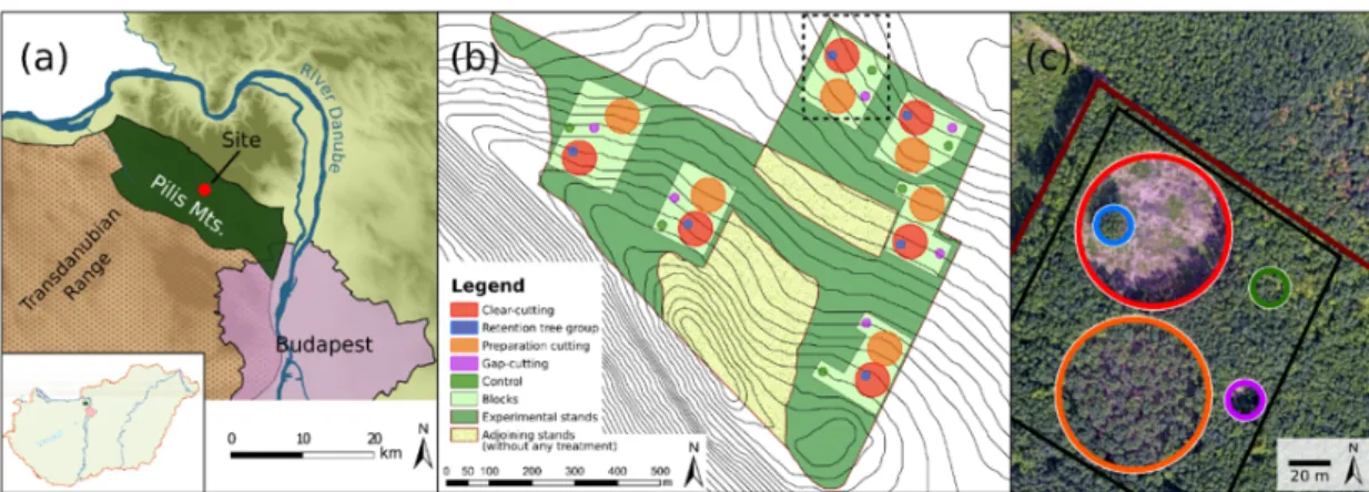
Figure 1. The study site of the Pilis Experiment in Northern Hungary. (a) Site location (47°40′ N, 18°54′
E) in the Pilis Mountains. (b) Experimental design showing the five treatments replicated within six blocks. (c) Aerial photograph revealing a block with the applied forestry treatments: clear-cutting (red) with a retention tree group (blue); preparation cutting (orange); gap-cutting (purple); and the control (green). Drone photo was taken by Viktor Tóth.
The bedrock consists of Dachsteinian limestone and Lattorfian sandstone with loess [51].
According to the soil profiles established in the study site, the soil depth varies along a slight topographic gradient (Supplementary Materials 1), deep (250 cm) at the lower elevations and shallow
Figure 1.The study site of the Pilis Experiment in Northern Hungary. (a) Site location (47◦400N, 18◦540 E) in the Pilis Mountains. (b) Experimental design showing the five treatments replicated within six blocks. (c) Aerial photograph revealing a block with the applied forestry treatments: clear-cutting (red) with a retention tree group (blue); preparation cutting (orange); gap-cutting (purple); and the control (green). Drone photo was taken by Viktor Tóth.
The bedrock consists of Dachsteinian limestone and Lattorfian sandstone with loess [51].
According to the soil profiles established in the study site, the soil depth varies along a slight topographic gradient (Supplementary Materials 1), deep (250 cm) at the lower elevations and shallow (70 cm) nearer the ridge. In the lower elevation parts of the site, the soil type is brown forest soil with clay illuviation (Luvisol), while in the upper parts it is Rendzic Leptosol [52]. The soils are slightly
Forests2018,9, 406 4 of 23
acidic (pH of the 0–20 cm layer is 4.6±0.2). The physical and chemical characteristics of the upper 50 cm of soil are similar in the whole area, independent of soil depth (Supplementary Materials 1).
The variety of soil types did not cause a discernible variability in the woody vegetation (Table1).
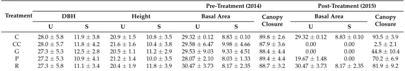
Table 1. Characteristics of forest structure around the plots, before and after treatments. Structural attributes (mean±standard deviation) presented here are the diameter at breast height ([DBH], cm), canopy height (m), basal area (m2ha−1), and canopy closure (%). U—upper layer; S—sub-canopy layer; C—control; CC—clear-cutting; G—gap-cutting; P—preparation cutting; R—retention tree group.
The mean and standard deviation were calculated based on the six replicates for each treatment type.
Treatment
Pre-Treatment (2014) Post-Treatment (2015)
DBH Height Basal Area Canopy
Closure
Basal Area Canopy Closure
U S U S U S U S
C 28.0±5.8 11.9±3.8 20.9±1.5 10.8±3.5 29.32±0.12 8.83±0.10 89.8±2.6 29.32±0.12 8.83±0.10 93.5±3.9 CC 28.0±5.7 11.8±4.2 21.6±1.6 10.4±3.8 29.58±6.47 9.98±4.66 87.9±3.6 0.00 0.00 2.5±2.1
G 27.3±5.3 12.5±2.8 20.5±1.1 11.2±2.9 29.53±9.03 9.33±4.51 88.4±4.4 0.00 0.00 44.8±10.4 P 27.2±5.3 10.9±4.1 21.2±1.4 10.0±3.5 28.07±2.10 8.03±1.33 89.4±4.4 19.67±1.48 0.00 70.2±6.9 R 27.3±5.8 11.1±3.4 20.4±1.9 11.8±3.9 30.47±3.73 8.17±2.35 88.7±3.2 30.47±3.73 8.17±2.35 81.9±9.2
The study site was established in an approximately 40 ha sized homogeneous unit, in a managed, two-layered sessile oak–hornbeam forest stand (Natura 2000 code: 91G0 [53]). The stand is even-aged (80 years old) and has a relatively uniform structure (Table1) and species composition, because of the applied shelterwood silvicultural system. The upper canopy layer (average height 21 m, mean diameter at breast height (DBH) 27.6 cm) is dominated by sessile oak, while the second most abundant tree species, hornbeam, forms a subcanopy layer with an average height of 11 m and a mean DBH of 11.6 cm (Table1and Figure S2.2). Other woody species are rare, and individuals ofFraxinus ornusL.,Fagus sylvaticaL.,Quercus cerrisL., andCerasus aviumL. were recorded in the tree layer as admixing tree species. Before the experimental treatments, the mean basal area (BA) of the upper layer was 29.4 (±4.3) m2 ha−1 and 8.8 (±2.6) m2 ha−1 in the case of the secondary canopy layer, respectively (Table1). The canopy closure was rather homogenous, varying between 81% and 94%.
The shrub layer was scarce and mainly consisted of the regeneration of hornbeam andFraxinus ornusL.
with a lower cover of shrub species (e.g.,Crataegus monogynaJacq.,Cornus masL.,Ligustrum vulgareL., andEuonymus verrucosusScop.). The understory layer was formed by general and mesic forest species.
Dominant species wereCarex pilosaScop.,Melica unifloraRetz.,Cardamine bulbiferaL.,Galium odoratum(L.) Scop., andGalium schultesiiVest. Before the treatments (in 2014), the herb layer cover was approximately 40%.
2.2. Study Design
Five treatment types (Figure S2.1) were implemented in a randomized complete block design in six replicates (hereafter blocks, Figure1b,c, and Table1):
1. Control (C): The original stand characteristics remained unaltered.
2. Clear-cutting (CC): Approximately 0.5 ha sized circular clear-cuts were formed, surrounded by a closed-canopy stand. The area of the treatment was designated as the area surrounded by the trunks of the peripheral dominant forest trees, the applied diameter was 80 m.
Within the clear-cuts, every tree individual (DBH≥5 cm and/or height≥2 m) was cut.
3. Gap-cutting (G): Circular artificial gaps were established in the closed stand by the elimination of all of the tree individuals within a diameter of 20 m (~0.03 ha). Gap size was defined as expanded gaps [54] (i.e., by measuring the base of surrounding canopy trees). The chosen 1:1 gap diameter/intact canopy height ratio is widely used in Central Europe for transition system applying gap-cutting, and it also fits well with the records of gap area in oak forests [55,56].
4. Preparation cutting (P): Uniform partial cutting was applied within a circle with a diameter of 80 m, and 30% of the initial total basal area of the upper canopy layer was cut in a spatially even arrangement. Furthermore, the complete subcanopy- and shrub-layer were also removed.
5. Retention tree group (R): All of the tree and shrub individuals were retained within a 0.03 ha sized circular plot (diameter = 20 m) in the clear-cuts, which resulted a small patch of the remained stand with approximately 8–12 trees of the former upper layer.
In accordance with the operative forestry law, individual clear-cuts in the submontane regions of Hungary are less than 5 ha [57]. The created clear-cuts are substantially smaller than it is typical in Hungary or in the temperate deciduous forests in Europe (3–10 ha). Therefore, changes in the site conditions resulting from this treatment may be less pronounced. In our experiment, neither the plots representing clear-cutting, nor the retention tree groups were placed in the center of the clear-cuts (Figure S2.2). These plots were shifted to the 1:3 intersections along the east–west axis, because we intended to minimize the bias caused by the shading of the remained trees of retention tree groups in the clear-cutting plots.
All of the treatments were carried out in the winter of 2014–2015. In the center of the treatments, a 6 m× 6 m fenced area (hereafter plot) was established to exclude the effects of the large-bodied game species.
2.3. Data Collection
Microclimate variables (total photosynthetic active radiation, air temperature, relative humidity, soil temperature, and soil moisture) were recorded every month of the growing season (March–October) of 2015 (directly after the implementation of the treatments). The litter and soil variables (litter mass, litter pH, litter moisture content, soil pH, hygroscopicity, and nutrient content) were measured in April and October of 2015.
Systematic microclimate measurements were taken in the center of each plot. Temporally synchronized data collection was carried out using 4-channeled Onset ‘HOBO H021-0020 data loggers (Onset Computer Corporation, Bourne, MA, USA) mounted on wooden poles (Figure S2.3).
Every month of the growing season (March–October), 72 h logging periods were applied with 10 min logging intervals. Photosynthetically active radiation (PAR, λ = 400–700 nm; µE m−2 s−1) was measured at 150 cm above ground level, using Onset ‘S-LIA-M0030quantum sensors (Onset Computer Corporation, Bourne, MA, USA). Air temperature (Tair; ◦C) and relative humidity (RH, %) data were collected 130 cm above ground level with Onset ‘S-THB-M0020(Onset Computer Corporation, Bourne, MA, USA) combined T/RH sensors (Onset Computer Corporation, Bourne, MA, USA) housed in standard radiation shields to avoid direct sunlight. The soil temperature (Tsoil;◦C) was measured with ‘S-TMB-M0020 12-Bit temperature sensors (Onset Computer Corporation, Bourne, MA, USA) by Onset placed 2 cm below ground. Soil water content (SWC; m3/m3) data were collected using Onset ‘S-SMD-M0050 soil moisture sensors (Onset Computer Corporation, Bourne, MA, USA) buried 20 cm below ground level to measure the average soil moisture at 10–20 cm soil depth. Air temperature and relative humidity data were used to calculate vapor pressure deficit (VPD; kPa) values at every logged occasion, following the protocol of Allen et al. [58], VPD = (0.6108){exp[17.27·Tair/(237.3 + Tair)]}·(1−RH/100). The reason for using VPD as a dependent variable is that it can give a direct indication of the atmospheric moisture conditions independently of the actual temperature. Therefore, it is a good standalone indicator of the atmospheric factors influencing evaporation; VPD describes the actual drying capacity of air (i.e., the higher the VPD is, the more intensive is the evaporation) [59]. Additionally, the relative diffuse light (DIFN; %) was measured using an LAI-2000 Plant Canopy Analyzer (LI-COR Inc., Lincoln, NE, USA) in the center of each plot at 130 cm above ground level. The measurements were carried out in August at dusk to avoid direct light affecting the sensor. Repeated measurements are not needed with this device [60].
A 270◦ view restrictor masked the portion of the sky containing the sun and the operator [61].
Reference above-canopy measuring was performed on an adjacent open field.
At each plot, four litter (30 cm × 30 cm area) and topsoil (0–20 cm depth) samples were systematically collected. All of the samples were returned to the laboratory and following the necessary preparation steps, and the litter mass, litter pH, litter moisture content, Kuron’s hygroscopicity (hy),
Forests2018,9, 406 6 of 23
soil organic matter content, and nutrient content were measured. The litter mass was measured after the samples were air-dried to a constant mass. The litter moisture content (%) was calculated as the mass loss of the freshly collected litter samples (i.e., the difference between the fresh and dried litter).
The litter and soil pH were potentiometrically measured using the supernatant suspension of air-dried and sieved (<2 mm) samples and 25 mL of distilled water, and the applied mass was 5 g for litter and 10 g for soil samples, respectively [62]. Kuron’s method was applied for gauging the hygrscopicity (hy) of air-dried soils [63], with a 50% (v/v) H2SO4solution and 35.2% RH, according to [62]. The chemical compounds were evaluated on the composite samples of the 1:1 mixture of the four sieved (<0.5 mm) subsamples per plot. The total soil carbon and nitrogen content were determined by dry combustion method using the Elementar vario MAX CNS-analyzer (Elementar Analysesysteme, Langenselbold, Germany), applying the International Organization for Standards (ISO) standards [64,65], as follows: the soil samples were weighed between 80 and 100 g, and a tungsten oxide catalyst was added. The applied combustion temperature was 1140◦C. Plant available phosphorus and potassium were determined by the ammonium lactate (AL) solution method (0.1 M NH4−lactate + 0.4 M HOAc, adjusted to pH 3.75), developed by Egnér et al. (1960, cf. [66]), according to the operative Hungarian standards [67]. The concentration of AL-soluble phosphorus (PAL) was measured colorimetrically, the concentration of AL-soluble potassium (KAL) was quantified by flame photometry.
All of the studied variables were also recorded in 2014 (pre-treatment conditions), applying the same methodology. The pre-treatment conditions of the plots selected for the different treatment levels were similar in 2014 (Table S3.1).
2.4. Data Analysis
The microclimate data were initially screened and the obvious errors caused by technical failures (indicated by, for example, unrealistic data or large spikes in variables) were replaced by missing values. The manually corrected data were imported into the database built in SpatiaLite 4.3.0a [68].
The observations were split into 24 h datasets. The differences from the values collected at the control were calculated for every recording (control values were subtracted from the treatment values of the block), and then the daily mean and interquartile range (IQR) of these difference values were computed.
To measure the direct effects of the silvicultural treatments on the site condition variables, these relative data were used to avoid the effects of actual weather conditions and local differences between the blocks.
For the analyses, one randomly chosen 24 h microclimate dataset was used every month. Daily IQR of the soil water content (SWC) was excluded from the analysis, because soil moisture is a rather stationary variable. For the relative humidity (RH) and vapor pressure deficit (VPD), as a result of numerous missing data, the subset of October was excluded.
The temporal patterns of the measured variables were investigated using two different temporal resolutions, according to the distinct methods for soil chemical variables and litter parameters, the seasons were compared (spring vs. autumn); while in the case of the microclimate variables, we used months as factor levels.
To explore the effect of the treatments and time on the measured site condition variables, linear mixed effects models (random intercept models) with a Gaussian error structure were used [69].
Where necessary, the data were transformed to achieve the normality of the model residuals. The effects of the different treatment levels across (1) the whole growing season and (2) over the applied temporal resolution (month or season) were tested by the same modeling framework, as follows: the treatment, time, and their interaction were used as fixed factors, while the block was specified as a random factor. The models’ goodness-of-fit values were measured by a likelihood-ratio test-based coefficient of determination (R2LR; [70]).The differences between the treatment levels were evaluated using the Tukey procedure (alpha = 0.05) for all of the pairwise comparisons. Multiple comparisons were applied to analyze the differences among the treatments throughout the growing season, based on the group means (‘glht’ function of ‘multcomp’ package; [71]), within the time levels on the least-squares means
(‘lsmeans’ function of ‘lsmeans’ package; [72]). The significance of the differences between the control and the other treatment levels was tested using linear mixed effects models, without intercept [73].
The diurnal patterns of the selected microclimate variables were shown using the original values (raw data). These were analyzed qualitatively, without any statistical test, applying the standard locally weighted scatterplot smoothing (LOWESS) analyses with 95% confidence intervals. The datasets were pooled into two groups, the peak of the growing season (i.e., June, July, and August) and the transitional period (March, April, September, and October) with lower canopy closure. Smoothing procedures were applied on 24 h datasets with six replicates for each treatment level.
The data analyses were performed using R version 3.4.1 [74]. inear mixed effects models were conducted by R package ‘nlme’ [75], and multiple comparisons were appraised using the ‘multcomp’ [71]
and ‘lsmeans’ [72] packages. The determination coefficients of the models were calculated using the ‘rsquaredLR’ function of the ‘MuMIn’ package [70]. For graphing, the modified script of the ‘errorbars’
function was used [76].
3. Results
3.1. The Effects of Experimental Treatments on Site Condition Variables
According to the performed linear mixed effects models (see Supplementary Materials 4 for details), we found that the experimental treatments affected microclimate and litter variables more, while the soil chemical characteristics did not differ significantly among treatment types—except for topsoil acidity (Table2and Figure2).
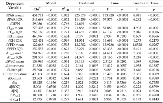
Table 2. The results of the linear mixed effects models performed for site condition variables.
PAR—photosynthetically active radiation (µE m−2 s−1); DIFN—relative diffuse light (%); Tair—air temperature (◦C); RH—relative humidity (%); VPD—vapor pressure deficit (kPa); Tsoil—soil temperature (◦C); SWC—soil moisture (m3/m3); Litter mass—total mass of collected litter on the surface (g/m2);
Litter pH—pH in water; Litter moisture content—gravimetric moisture content of litter samples (%);
Soil pH—soil pH in water; hy—Kuron’s hygrscopicity (%); [SOC]—total soil carbon content (%);
[N]—total nitrogen content (%); [PAL]—concentration of AL-soluble phosphorus (mg/100 g soil);
[KAL]—concentration of AL-soluble potassium (mg/100 g soil).drefers to the difference from the values measured in the control plots. For modeling, 24 h means were used, except in the case of PAR, where the daytime (6:00–18:00 Coordinated Universal Time [UTC]) means were calculated.
Dependent Variable
Model Treatment Time Treatment: Time
Chi2 p R2LR F p F p F p
dPAR mean 454.711 <0.0001 0.922 225.579 <0.0001 133.928 <0.0001 8.941 <0.0001 dPAR IQR 343.698 <0.0001 0.852 114.259 <0.0001 57.575 <0.0001 6.292 <0.0001
dDIFN 29.086 <0.0001 0.766 21.699 <0.0001 - - - -
dTairmean 273.305 <0.0001 0.781 21.888 <0.0001 54.082 <0.0001 4.903 <0.0001 dTairIQR 265.160 <0.0001 0.771 44.487 <0.0001 47.139 <0.0001 2.016 0.0086 dRH mean 46.096 <0.0001 0.434 5.177 0.0021 2.939 0.0105 0.609 0.8866 dRH IQR 125.451 <0.0001 0.569 14.054 <0.0001 16.694 <0.0001 1.275 0.2173 dVPD mean 122.668 <0.0001 0.595 13.2782 <0.0001 13.9286 <0.0001 1.8528 0.0267 dVPD IQR 259.555 <0.0001 0.823 37.279 <0.0001 63.435 <0.0001 5.491 <0.0001 dTsoilmean 261.975 <0.0001 0.768 9.107 <0.0001 44.611 <0.0001 7.368 <0.0001 dTsoilIQR 201.537 <0.0001 0.674 24.397 <0.0001 24.166 <0.0001 3.248 <0.0001 dSWC mean 109.965 <0.0001 0.534 29.145 <0.0001 2.3129 0.0292 1.089 0.3666 dLitter mass 21.338 0.0033 0.424 2.164 0.1097 10.812 0.0057 1.955 0.1387 dLitter pH 35.390 <0.0001 0.524 8.888 0.0002 8.685 0.0057 3.646 0.0218 dLitter moisture 47.003 <0.0001 0.624 9.318 0.0001 16.478 0.0003 7.355 0.0009 dSoil pH 23.863 0.0012 0.544 3.633 0.0221 15.754 0.0003 0.041 0.9889
dhy 10.428 0.1656 0.219 2.824 0.0528 0.115 0.7369 0.426 0.7358
d[SOC] 5.008 0.6590 0.352 1.202 0.3242 0.159 0.6930 0.223 0.8799
d[N] 3.415 0.8442 0.357 0.912 0.4451 0.008 0.9316 0.074 0.9738
d[PAL] 10.308 0.1718 0.388 1.936 0.1418 1.034 0.3163 0.965 0.4200 d[KAL] 12.735 0.0788 0.299 1.641 0.1821 6.956 0.0124 0.173 0.9143
Forests2018,9, 406 8 of 23
Forests 2018, 9, x FOR PEER REVIEW 9 of 24
Figure 2. Changes in means and interquartile ranges (IQR) of the relative values of the site condition variables among the forestry treatments in Pilis Mountains, Hungary, 2015. (a) Mean and (b) IQR of photosynthetically active radiation (PAR; μE m−2 s−1); (c) mean of relative diffuse light (DIFN; %); (d) mean and (e) IQR of air temperature (Tair; °C); (f) mean and (g) IQR of relative humidity (RH; %); (h) mean and (i) IQR of vapor pressure deficit (VPD; kPa); (j) mean and (k) IQR of soil temperature (Tsoil;
°C); (l) mean of soil moisture (SWC; m3/m3); (m) total mass of collected litter on the surface (g/m2); (n) litter pH (pH in water); (o) gravimetric moisture content of litter samples (%); (p) soil pH (pH in water). The letter ‘d’ in the variable abbreviations refers to the differences from the mean values measured in the control plots. The treatment types are coded as follows: CC—clear-cutting; G—gap- cutting; P—preparation cutting; R—retention tree group. Full circles show the mean and vertical lines denote the standard deviation of the samples. Letters designate the significant differences among the treatments (all of the pairwise multiple comparisons based on the linear mixed effects models; Tukey- test, alpha = 0.05), while asterisks denote significant differences from the values measured at the control plots (linear mixed effects models without intercept, p < 0.05). The horizontal blue line shows the level of the control.
3.2. Temporal Differences among Treatments through the Growing Season
Besides the study of the treatment effects, the temporal differences during a growing season were also analyzed (Table 2). Except for the light and soil moisture variables, the effect of time was similar or stronger than that of treatments. For the litter mass and potassium content, only the effect of time was significant.
The largest differences in the microclimate variables were detectable in summer (Figure 3). dPAR was the highest in the clear-cuts in almost every month, but the differences were the highest in full- leaved months—from May to August (Figure 3a). The dVPD values were highly divergent among
Figure 2.Changes in means and interquartile ranges (IQR) of the relative values of the site condition variables among the forestry treatments in Pilis Mountains, Hungary, 2015. (a) Mean and (b) IQR of photosynthetically active radiation (PAR;µE m−2s−1); (c) mean of relative diffuse light (DIFN; %);
(d) mean and (e) IQR of air temperature (Tair;◦C); (f) mean and (g) IQR of relative humidity (RH; %);
(h) mean and (i) IQR of vapor pressure deficit (VPD; kPa); (j) mean and (k) IQR of soil temperature (Tsoil;◦C); (l) mean of soil moisture (SWC; m3/m3); (m) total mass of collected litter on the surface (g/m2); (n) litter pH (pH in water); (o) gravimetric moisture content of litter samples (%); (p) soil pH (pH in water). The letter ‘d’ in the variable abbreviations refers to the differences from the mean values measured in the control plots. The treatment types are coded as follows: CC—clear-cutting;
G—gap-cutting; P—preparation cutting; R—retention tree group. Full circles show the mean and vertical lines denote the standard deviation of the samples. Letters designate the significant differences among the treatments (all of the pairwise multiple comparisons based on the linear mixed effects models; Tukey-test, alpha = 0.05), while asterisks denote significant differences from the values measured at the control plots (linear mixed effects models without intercept,p< 0.05). The horizontal blue line shows the level of the control.
The mean (Figure2a) and the IQR (Figure2b) of photosynthetic active radiation (dPAR), as well as the mean of relative diffuse light (dDIFN, Figure2c) were substantially higher in all of the treatments than in the controls. The largest values were detected in the clear-cuts, and the increment was also considerable in the gap-cuts. The light conditions were similar in the preparation cuts and the retention tree groups, but the dDIFN was lower in the retention tree groups. The mean and interquartile range of the air temperature (dTair) departed significantly from the control in all of the treatments (Figure2d,e). In the retention tree groups and clear-cuts, the mean of thedTairwas significantly higher than in the other two treatments (Figure2d). ThedTairwas buffered the most in the preparation cuts,
but the mean ofdTair was not different from that in the gap-cuts. Both the mean and the standard deviation of the IQR were the highest in the clear-cuts (Figure2e). The lowest IQR was measured in the gap-cuts, while in the other treatments, the IQR was intermediate. The mean of relative humidity (dRH) was the lowest in the clear-cuts and in the retention tree groups (Figure2f). In the preparation cuts and gap-cuts, the humidity remained similar to the control; furthermore, these treatments did not differ from each other. It is noticeable that the IQR of thedRH was the lowest in the gap-cuts and the highest in the clear-cuts, however, in all of the treatments, the IQRs of thedRH were departed from the control (Figure2g). The mean and IQR of the vapor pressure deficit (dVPD) showed the same pattern asdTair, because of the high contribution of temperature to this variable, and all of the treatments also differed significantly from the control (Figures2h and2i, respectively). The mean and IQR of the soil temperature (dTsoil) differed significantly in every treatment from the control (Figures2j and 2k, respectively). The clear-cutting created soil thermal conditions that divaricated the most from those in the closed stand; both the mean and IQR of thedTsoilwere the highest there. In the retention tree groups, the mean of thedTsoildid not differ significantly from that of the clear-cuts, but the IQR was significantly lower there. The coolest soil environment with the lowest IQR was detected in the gap-cuts.
The soil moisture (dSWC) differed significantly in the clear-cuts and even more in the gap-cuts from that in the controls (Figure2l). The highestdSWC was measured in the gap-cuts, the increase was smaller in the clear-cuts, while a slight decrease was detected in the preparation cuts and in the retention tree groups, and the latter was the driest treatment.
The litter variables showed a strong response to the treatments (Table2). In the first year, there was no significant response in the litter mass, however, it showed an increasing trend from the clear-cutting to the retention tree group (Figure2m). In the clear-cuts and in the gap-cuts, the litter pH departed significantly from that in the controls, and the litter were more neutral in these two treatments than in the preparation cuts and in the retention tree groups (Figure 2n). The litter moisture followed the sequence ofdSWC. The forest floor was the driest in the retention tree group, but it was not significantly different from that in the controls, and the litter moisture was significantly higher in the other three treatments—the highest values were measured in the gap-cuts (Figure2o). Among the soil variables, only the soil pH showed a significant treatment effect, the topsoil was less acidic in the preparation cuts than in the other treatments and it was the only treatment level where the soil pH differed from the control (Table2, Figure2p).
3.2. Temporal Differences among Treatments through the Growing Season
Besides the study of the treatment effects, the temporal differences during a growing season were also analyzed (Table2). Except for the light and soil moisture variables, the effect of time was similar or stronger than that of treatments. For the litter mass and potassium content, only the effect of time was significant.
The largest differences in the microclimate variables were detectable in summer (Figure3).dPAR was the highest in the clear-cuts in almost every month, but the differences were the highest in full-leaved months—from May to August (Figure3a). ThedVPD values were highly divergent among the treatment levels during summer, the drying capacity of air was significantly higher in the clear-cuts and in the retention tree groups, while thedVPD did not depart substantially from the control in the case of the two other treatment types (Figure3b).dTsoilwas the largest in the clear-cuts with the highest variance during the summer (Figure3c); the differences between the treatment levels accelerated as the canopy closure increased, but gap-cutting and preparation cutting created similar conditions to the control during the whole growing season. The retention tree group could partly buffer thedTsoil. As the first frosts appeared (in October), thedTsoil differed significantly from the other treatments in the clear-cuts (i.e., the soil was the coldest there). ThedSWC increment in the gap-cuts was detectable through the whole measurement period, and it increased during summer (Figure3d). It was also relatively high in the clear-cuts, but the difference was less pronounced than that in the gap-cuts. A moderate soil desiccation was detected in the retention tree groups from June to September.
Forests2018,9, 406 10 of 23
Forests 2018, 9, x FOR PEER REVIEW 11 of 24
Figure 3.Temporal variability of the selected microclimate variables among the experimental treatments and months in the Pilis Mountains, Hungary, 2015. (a) Mean of the photosynthetically active radiation ([PAR]µE m−2s−1); (b) mean of vapor pressure deficit ([VPD] kPa); (c) mean of soil temperature ([Tsoil]
◦C); (d) mean of soil moisture ([SWC] m3/m3). The letterdin the variable abbreviations refers to the differences from the mean values measured in the control plots. Treatment types are coded as follows:
CC—clear-cutting; G—gap-cutting; P—preparation cutting; R—retention tree group. Full circles show the mean and vertical lines denote the standard deviation of the samples. Letters designate the significant differences among the treatments and months (all of the pairwise multiple comparisons based on the linear mixed effects models: Tukey test, alpha = 0.05). The horizontal blue line shows the level of the control.
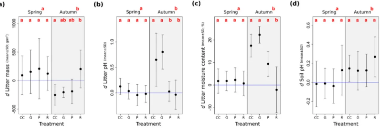
The litter mass decreased from spring to autumn in the treatments, except for the retention tree group (Figure4a). The litter pH increased in the gap-cuts and in the clear-cuts in autumn, while in the preparation cuts and in the retention tree groups, it stayed close to the values that had been measured in the uncut controls (Figure4b). The litter moisture content increased marginally in the preparation cuts and more markedly in the clear-cuts, as well as in the gap-cuts, as compared to the degree of humidity measured in spring (Figure4c). We found that the effect of time was significant for pH and KAL-concentration (Table2). The soil pH was lower in spring than in autumn, and in both periods, it was higher in the retention tree groups than in the other treatments (Figure4d).
Figure 3. Temporal variability of the selected microclimate variables among the experimental treatments and months in the Pilis Mountains, Hungary, 2015. (a) Mean of the photosynthetically active radiation ([PAR] μE m−2 s−1); (b) mean of vapor pressure deficit ([VPD] kPa); (c) mean of soil temperature ([Tsoil] °C); (d) mean of soil moisture ([SWC] m3/m3). The letter d in the variable abbreviations refers to the differences from the mean values measured in the control plots. Treatment types are coded as follows: CC—clear-cutting; G—gap-cutting; P—preparation cutting; R—retention tree group. Full circles show the mean and vertical lines denote the standard deviation of the samples.
Letters designate the significant differences among the treatments and months (all of the pairwise multiple comparisons based on the linear mixed effects models: Tukey test, alpha = 0.05). The horizontal blue line shows the level of the control.
Figure 4. Seasonal changes in selected soil and litter variables in Pilis Mountains, Hungary, 2015. (a) Total mass of collected litter on the surface (g/m2); (b) litter pH (pH in water); (c) gravimetric moisture content of litter samples (%); (d) soil pH (pH in water). The letter d in the variable abbreviations refers to the differences from the mean values measured in the ‘Control’ plots. Treatment types are coded as follows: CC—clear-cutting; G—gap-cutting; P—preparation cutting; R—retention tree group. Full circles show the mean and vertical lines denote the standard deviation of the samples. Letters designate the significant differences among the treatments (all of the pairwise multiple comparisons based on the linear mixed effects models; Tukey test, alpha = 0.05). The horizontal blue line shows the level of the control.
3.3. Diurnal Pattern of Microclimate Variables among the Treatments
When we analyzed the 24-h datasets, a clear diurnal pattern could be detected for the different microclimate variables with large variability between the treatments in summer (Figure 5).
Contrarily, when the pooled early spring and autumn subsets were analyzed, differences were much smaller and the pattern was not as obvious.
Figure 4. Seasonal changes in selected soil and litter variables in Pilis Mountains, Hungary, 2015.
(a) Total mass of collected litter on the surface (g/m2); (b) litter pH (pH in water); (c) gravimetric moisture content of litter samples (%); (d) soil pH (pH in water). The letterdin the variable abbreviations refers to the differences from the mean values measured in the ‘Control’ plots. Treatment types are coded as follows:
CC—clear-cutting; G—gap-cutting; P—preparation cutting; R—retention tree group. Full circles show the mean and vertical lines denote the standard deviation of the samples. Letters designate the significant differences among the treatments (all of the pairwise multiple comparisons based on the linear mixed effects models; Tukey test, alpha = 0.05). The horizontal blue line shows the level of the control.
3.3. Diurnal Pattern of Microclimate Variables among the Treatments
When we analyzed the 24-h datasets, a clear diurnal pattern could be detected for the different microclimate variables with large variability between the treatments in summer (Figure 5).
Contrarily, when the pooled early spring and autumn subsets were analyzed, differences were much smaller and the pattern was not as obvious.
The PAR differed considerably between the treatments in summer. It frequently exceeded 2000µE m−2s−1in the clear-cuts, while in the second brightest plots, in the gap-cuts, the maximum values were under 1930 µE m −2 s−1. There was a detectable lag of the maximum values as follows: in the clear-cuts, it appeared at 12:00–12:20 Coordinated Universal Time (UTC); at around 12:30–12:40 UTC in the gap-cuts; and at 13:10–13:20 UTC in the preparation cuts. In the retention tree groups, the maximum values occurred between 9:00 and 10:30 UTC. This was followed by a decrease in radiation because of the shading effect of the canopy patch. The pattern of irradiance among the treatments was also detectable in the case of VPD and Tsoil, for instance, in the morning, the retention tree group was the warmest and driest treatment. In the clear-cuts, it sometimes reached 38.8◦C in summer, but even in the retention tree groups, its maximum was 31.3◦C. In the gap-cuts, the moist soil (dSWC) was the highest (Figure2l), resulting in a distinct peak in VPD, which was followed by a quick decrease; and the Tsoilwas lower, despite the high PAR. The clear-cuts cooled down the most in the summer, between 2:00 and 7:30 am, and especially in the transitional period. In the transition period, the amplitudes of the diurnal cycles were substantially smaller. Furthermore, the microclimate within the applied treatments did not differ as much as during the peak of the growing season as it did during the other seasons.
Forests2018,9, 406 12 of 23
Forests 2018, 9, x FOR PEER REVIEW 13 of 24
Figure 5. Diurnal patterns of selected microclimate variables. Diurnal magnitudes of PAR (photosynthetically active radiation), VPD (vapor pressure deficit) and Tsoil (soil temperature) among treatments in the peak of the growing season (i.e., June, July, August; left) and during the transition period (March, April, September, October; right), respectively. Lines represent means calculated by LOWESS function (based on the 6 replicates for each variable per month), bands represent 95%
confidence intervals. Colors are coding the treatments: control—green; clear-cutting—red; gap- cutting—purple; preparation cutting—orange and retention tree group—blue. Note that scales of y- axes vary between graphs.
The PAR differed considerably between the treatments in summer. It frequently exceeded 2000 μE m−2 s−1 in the clear-cuts, while in the second brightest plots, in the gap-cuts, the maximum values were under 1930 μE m −2 s−1. There was a detectable lag of the maximum values as follows: in the clear-cuts, it appeared at 12:00–12:20 Coordinated Universal Time (UTC); at around 12:30–12:40 UTC in the gap-cuts; and at 13:10–13:20 UTC in the preparation cuts. In the retention tree groups, the maximum values occurred between 9:00 and 10:30 UTC. This was followed by a decrease in radiation because of the shading effect of the canopy patch. The pattern of irradiance among the treatments was also detectable in the case of VPD and Tsoil, for instance, in the morning, the retention tree group was the warmest and driest treatment. In the clear-cuts, it sometimes reached 38.8 °C in summer, but even in the retention tree groups, its maximum was 31.3 °C. In the gap-cuts, the moist soil (dSWC) was the highest (Figure 2l), resulting in a distinct peak in VPD, which was followed by a quick decrease; and the Tsoil was lower, despite the high PAR. The clear-cuts cooled down the most in the
Figure 5. Diurnal patterns of selected microclimate variables. Diurnal magnitudes of PAR (photosynthetically active radiation), VPD (vapor pressure deficit) and Tsoil(soil temperature) among treatments in the peak of the growing season (i.e., June, July, August; left) and during the transition period (March, April, September, October; right), respectively. Lines represent means calculated by LOWESS function (based on the 6 replicates for each variable per month), bands represent 95% confidence intervals. Colors are coding the treatments: control—green; clear-cutting—red;
gap-cutting—purple; preparation cutting—orange and retention tree group—blue. Note that scales of y-axes vary between graphs.
4. Discussion
4.1. Rapid Changes in Microclimate and Litter Variables, but Not in Soil Properties
In general, and in accordance with our expectations, the microclimate variables showed strong short-term deviations among the different silvicultural treatments. Interestingly, the litter characteristics also changed in the first growing season. As presumed, we could not demonstrate significant changes for most of the investigated soil variables (physical or chemical). Two different, but highly interrelated processes can be highlighted in the context of microclimate alteration by forest management, radiation balance and evapotranspiration. The forest canopy plays an important role in both of the mechanisms.
The maintenance of the buffered microclimate in the below-canopy space of the closed forest stands is based on the shielding effect, namely, through the (partial) shading and the absorption of the
foliage, there is significantly less net radiation to heat the forest floor. Moreover, the canopy insulates the understory environment by reducing the longwave radiative loss [19,26,43]. Furthermore, as demonstrated by Bristow and Campbell [77], there is a strong correlation between solar irradiance and transferred heat-related variables of the ambient air, such as air temperature, relative humidity, and vapor pressure deficit. This may explain why, in the harvested sites, we measured a generally higher and temporally more variable irradiance, temperature, and vapor pressure deficit, and a lower, but also more unbalanced air humidity. The changes in the soil moisture following the different treatments are based (1) on the lower rate of interception and evaporation through the canopies or trunks and, consequently, the increased throughfall; and (2) on the lower transpiration rates due to tree removal [32,78,79]. The major effect of these alterations is that the soil water content typically increases in sites where felling was applied on to larger continuous extent (i.e., in gap-cuts and clear-cuts).
4.1.1. Light Variables
As the applied treatments mainly modified the canopy closure of the stand, the (1) total and diffuse light departed from the control in every treatment because of the harvest-induced canopy modifications, and (2) the light variables had the strongest response to the treatments. Our findings are congruent with previous research, showing that the increment in irradiance and its variability highly correlate with the increase of canopy openings and the leaf area index [19,22,33,35]. Therefore, solar radiation is higher and temporally more variable in the clear-cuts than that in the forest edges [80], in the stands harvested by various types of green tree retention schemes [36] or in the management practices related to the uneven-aged systems [8].
The canopy gaps also create a more illuminated environment [81–83], although the irradiance was significantly lower than that detected in the clear-cuts, because of the smaller sky view factor [35] and consequently, the shading of the surrounding trees [41]. The preparation cuttings and retention tree groups did not show clear differences in the light level and its variance. These treatments engender a similarly brighter environment than the uncut sites [36,84,85].
The spatial arrangement of the trees influenced the direct-diffuse light proportions.
In the preparation cuts, the uniform distribution of the trees strongly inhibited the direct irradiation, but less notably the diffuse light. Therefore, interestingly, the amount of the diffuse light is similar to that in the gap-cuts, but the amount of total irradiance is significantly lower [83,86]. The retention tree group—in the first year—was very open to the adjacent clear-cutting and to the lateral irradiance because of the lack of lower branches and the sparse shrub layer. However, we can expect that the illumination in the retention tree groups will decrease and return to the level characteristic in the control, as the natural regeneration (shrubs, sprouts, and juvenile trees) grows and as the epicormic shoots emerge.
4.1.2. Air Variables
Forest management (especially clear-cutting) has a strong and long-lasting effect on air temperature and relative humidity [87,88]; silvicultural interventions could generate alterations in these variables that persist over 25 years. Contrary to previous studies reporting that the temperature and humidity in the stands harvested using moderately intensive management practices had only slightly modified microclimates compared to the uncut plots (e.g., thinning [42], group selection [89], and gaps [79]), we found that almost every treatment type resulted significant departures from the control in these variables. However, our treatments resulted similar trends in the Tair, RH, and VPD changes, as found in other studies (e.g., [36,44,81,90]).
Since the highest levels of incoming solar radiation were measurable in the clear-cuts, this treatment type can be characterized by the highest air temperature and vapor pressure deficit, as well as the lowest relative humidity values [20,32,36]. Our findings are in agreement with the results of Carlson and Groot [35] and von Arx et al. [21], that the increment of Tairconcerning the whole growing season was less than 1◦C in the clear-cuts. The differences in the Tair or RH between the clear-cuts and the closed stands were higher in many studies that investigated the impacts of larger
Forests2018,9, 406 14 of 23
clearings. In our experiment, because of the relatively small size (0.5 ha) of the clear-cuts, the shading effect of the forest edge, as well as the cooling effect by mixing air from the nearby stand, may have been be more pronounced [91–93].
The mean Tair and VPD in the gap-cuts were significantly lower than those in the clear-cuts or the retention tree groups, regardless of the high PAR values and the observed generally strong correlation between direct radiation and air temperature in the gaps [81]. This could be explained by the high soil moisture and evaporative cooling in the gap-cuts [26,94]. The mean increment in temperature (~0.1◦C) was comparable with the studies of Carlson and Groot [35], or Abd Latif and Blackburn [83]. The air humidity may have remained unaltered in the gaps because of the lower ratio of air mixing and the shading by the adjacent closed stands [19,83], and the moist topsoil as a source of water vapor [28].
The thermal conditions of the preparation cutting (where 70% of the original BA was retained) were similar to the gap-cutting. The mean of VPD and RH in the preparation cuts remained similar to that in the controls, but the ranges of these variables departed because of the higher input of solar energy and the lack of subcanopy and shrub-layers [27,42].
We expected that the retention tree group in the clear-felled area would substantially buffer the thermal effects created by clear-cutting, as was measurably the case for the light variables.
However, it was found that the retention tree groups did not compensate for the thermal loading and the drying capacity of the warmer air coming from the clearings, the mean of the Tairand VPD were not significantly different from those of the clear-cutting. This phenomenon could be due to the edge effect (in the case of the Tair, VPD, and RH), given the relatively small applied patch size [80,92,93,95].
In contrast, the retention tree group successfully reduced the variability (IQR) and the extreme values of these variables by the insulation of the remained canopy patch, in spite of the effective lateral mixing [95,96].
4.1.3. Soil Temperature
Increased the incoming solar radiation caused a significant increment in the soil temperature (both in the case of the means and IQRs) in all of the treatments. Higher departures from the control levels were measured than in the case of the air temperature, because of the less pronounced moderating effect of the canopy [26]. According to the strong correlation between Tairand Tsoil[97,98], the decreasing trends of these variables across the treatments were similar. Implicitly, because of the enhanced solar heating in daytime and the longwave radiation loss in nighttime, clear-cutting showed the greatest increase in the mean and variability of Tsoil[21,35,91]. The retention tree group may have moderated the extremes of Tsoilbetter than Tairbecause of the shading provided by the remaining trees. These are similar to the results of Williams-Linera and colleagues, who investigated the impacts of isolated trees [99], but in our case, we detected a more pronounced smoothing effect in the variability of Tsoil. Interestingly, the range of Tsoilin the retention tree groups was comparable with that measured in the preparation cuts and in the gap-cuts. In the gap-cuts and in the preparation cuts, we recorded a smaller increase in Tsoilthan has been reported in previous studies [13,81–83].
4.1.4. Soil Moisture
The forest stands are characterized by high evapotranspiration rates; therefore, in general, any opening in the canopy results in a reduction of the amount of water that is utilized and intercepted [33,78]. The impact of the elimination of the tree individuals is particularly significant on the moisture content of the upper layer of the forest soil [32,81]. As expected, the clear-cutting and gap-cutting also induced a significant increase in the soil moisture levels when compared with the controls, because of the drastic decrease of the transpiring surface [19,41,81–83]. However, although the relative contribution of transpiration to evapotranspiration is higher than the proportion of soil evaporation [78], the greatest increment was detectable in the gap-cuts. The smaller increase in the clear-cuts can be explained by enhanced irradiation, which accelerates the evaporation from