1
This manuscript is contextually identical with the following published paper: Kovács, B., Tinya, F., 1
Németh, Cs. and Ódor, P. 2020. Unfolding the effects of different forestry treatments on microclimate 2
in oak forests: results of a 4-year experiment. Ecological Applications 30(2): e02043. The original 3
article is published at https://doi.org/10.1002/eap.2043.
4 5
Running head: Management-induced microclimate changes 6
7
Unfolding the effects of different forestry treatments on microclimate in oak forests: results 8
of a 4-year experiment 9
10
Bence Kovács1,2,3,*, Flóra Tinya1, Csaba Németh2, Péter Ódor1,2 11
12
1 MTA Centre for Ecological Research, Institute of Ecology and Botany, Alkotmány út 2-4, H- 13
2163 Vácrátót, Hungary 14
2 MTA Centre for Ecological Research, GINOP Sustainable Ecosystems Research Group, 15
Klebelsberg Kuno utca 3, H-8237 Tihany, Hungary 16
3 Department of Plant Systematics, Ecology and Theoretical Biology, Eötvös Loránd University, 17
Pázmány Péter sétány 1/C, H-1117 Budapest, Hungary 18
19
* Corresponding author: kovacs.bence@okologia.mta.hu; Tel.: +36-28-360-122/107 20
21 22 23 24
2 25
3 Abstract
26
Stable below-canopy microclimate of forests is essential for their biodiversity and ecosystem 27
functionality. Forest management necessarily modifies the buffering capacity of woodlands.
28
However, the specific effects of different forestry treatments on site conditions, the temporal 29
recovery after the harvests and the reason of the contrasts between treatments are still poorly 30
understood.
31
The effects of four different forestry treatments (clear-cutting, retention tree group, preparation 32
cutting and gap-cutting) on microclimatic variables were studied within a field experiment in a 33
managed oak dominated stand in Hungary, before (2014) and after (2015–2017) the 34
interventions by complete block design with six replicates.
35
From the first post-treatment year, clear-cuts differed the most from the uncut control due to the 36
increased irradiance and heat load. Means and variability of air and soil temperature increased, 37
air became dryer along with higher soil moisture levels. Retention tree groups could effectively 38
ameliorate the extreme temperatures but not the mean values. Preparation cutting induced slight 39
changes from the original buffered and humid forest microclimate. Despite the substantially 40
more incoming light, gap-cutting could keep the cool and humid air conditions and showed the 41
highest increase in soil moisture after the interventions. For most microclimate variables, we 42
could not observe any obvious trend within three years. Though soil temperature variability 43
decreased with time in clear-cuts, while soil moisture difference continuously increased in gap- 44
and clear-cuts. Based on multivariate analyses, the treatments separated significantly based 45
mainly on the temperature maxima and variability.
46
4
We found that (i) the effect sizes among treatment levels were consistent throughout the years;
47
(ii) the climatic recovery time for variables appears to be far more than three years and (iii) the 48
applied silvicultural methods diverged mainly among the temperature maxima.
49
Based on our study, the spatially heterogeneous and fine-scaled treatments of continuous cover 50
forestry (gap-cutting, selection systems) are recommended. By applying these practices, the 51
essential structural elements creating buffered microclimate could be more successfully 52
maintained. Thus, forestry interventions could induce less pronounced alterations in 53
environmental conditions for forest-dwelling organism groups.
54 55 56 57
Keywords: air temperature;forest ecological experiment; forest management; photosynthetically 58
active radiation (PAR); relative humidity; soil moisture; soil temperature; temperate deciduous 59
forests; vapor pressure deficit (VPD) 60
61 62 63
5 Introduction
64
Microclimate studies as well as the integration of their outcomes into climate-dependent 65
models have become an important research area for both climatologists, ecologists and 66
practitioners in the last two decades. This topic is especially relevant facing the current 67
anthropogenic climate change and its effects on ecosystems and their functionality (Hannah et al.
68
2014, Frey et al. 2016, Bramer et al. 2018). The better understanding of microclimate can 69
contribute to the adjustment of climate and species distribution models. It has been revealed 70
since decades that organisms are exposed to the variability of climate on finer spatial scales than 71
it is typically measured by standard meteorological stations worldwide (Geiger et al. 1995, Potter 72
et al. 2013). This mismatch results in coarser scale abiotic data that are not entirely appropriate 73
for surveying and modelling biological processes (Suggitt et al. 2011, De Frenne and Verheyen 74
2016). Furthermore, local conditions can often result in microclimates that are substantially 75
different from the macroclimate; therefore, the ranges of the driving forces of species distribution 76
– e.g., climatic extremes – are narrowed (Suggitt et al. 2011, Scherrer et al. 2011, Scheffers et al.
77
2014). As a result, the lack of information about the upper or lower limits could cause either 78
over- or underprediction of the climatically suitable microenvironments for species (Ashcroft 79
and Gollan 2013, Hannah et al. 2014, Frey et al. 2016). Though woodlands have been identified 80
as a main factor shaping climatic microrefugia besides topography and moisture conditions 81
(Ashcroft and Gollan 2013, von Arx et al. 2013, Latimer and Zuckerberg 2017), there are still 82
limited data collected beneath forest canopies which would be essential for climatic predictions 83
as well as species distribution modelling (De Frenne and Verheyen 2016, Bramer et al. 2018).
84
Hence, it is necessary to explore the below-canopy microclimates in stand types, which are 85
6
different based on physiography, forest site conditions, tree species composition, vertical and 86
horizontal structure or natural and anthropogenic disturbance regimes.
87
It is widely known that forests create unique, stable and ameliorated below-canopy 88
microclimates which substantially differ from the adjoining open habitats (Geiger et al. 1995, 89
Chen et al. 1999, von Arx et al. 2012, Barry and Blanken 2016). In the trunk space, the mean and 90
variance of air and soil temperature are typically lower. Similarly, the vapor pressure deficit or 91
wind velocity is reduced, while the air humidity is higher than these characteristics in open-field.
92
This special buffered environment was proved to be an essential driver of biodiversity as well as 93
numerous biogeochemical processes and ecosystem functionality (Lewandowski et al. 2015, 94
Good et al. 2015, Ehbrecht et al. 2017, Davis et al. 2018). Among others, microclimate was 95
revealed as an important factor of vitality and survival of woodland herbs (Lendzion and 96
Leuschner 2009), species composition and community structure of understory vegetation (Aude 97
and Lawesson 1998, Godefroid et al. 2006, De Frenne et al. 2015), the frost sensibility of 98
saplings (von Arx et al. 2013, Charrier et al. 2015), the richness, abundance or vertical 99
occurrence of cryptogams (Coxson and Coyle 2003, Gaio-Oliveira et al. 2004, Fenton and Frego 100
2005, Dynesius et al. 2008), the species composition of spiders and saproxylic beetles (Košulič 101
et al. 2016, Seibold et al. 2016) and also the survival and population density of forest-inhabiting 102
birds (Betts et al. 2018).
103
The canopy cover and its structure are typically highlighted as one of the most important 104
drivers of the buffer capacity of a given forest stand (Bonan 2016, Latimer and Zuckerberg 2017, 105
De Frenne et al. 2019), which is necessarily altered by forest management practices (Chen et al.
106
1999, Hardwick et al. 2015, Lin et al. 2017, Ehbrecht et al. 2019). Forestry interventions creating 107
for example clear-felled areas or stands with large openings generate microclimatic conditions 108
7
which are considerably different from those in forests (Chen et al. 1999, Bonan 2016).It is an 109
important conservational aspect to study how these management types induced alterations affect 110
the climatically suitable habitats for forest-dwelling organism groups (De Frenne and Verheyen 111
2016). Furthermore, regeneration time of microclimatic conditions after anthropogenic 112
disturbances generated by silviculture is also a highly relevant question for the colonization (or 113
recovery) of forest-dwelling populations.
114
Forest management (especially clear-cutting) could have long-term effects on light regime, 115
moisture conditions of the forest soil, air temperature and humidity as well as vapor pressure 116
deficit. Changes in the environmental conditions after clear-cutting can persist over years or 117
decades whereupon microclimate can recover to pre-treatment levels (Matlack 1993, Dodonov et 118
al. 2013, Dovčiak and Brown 2014, Baker et al. 2014). In contrary, the observed alterations 119
following partial harvesting methods or gap-cutting are described usually as ephemeral processes 120
(Aussenac and Granier 1988, Anderson et al. 2007, Grayson et al. 2012). However, there is still 121
limited knowledge about the temporal climatic recovery after forestry interventions in Europe.
122
Beside the general and temporal effects of silvicultural management on forest microclimate, it 123
is also important to identify the most influential microclimatic variables that generate differences 124
between the certain forestry treatments. Many studies underline that forest-dwelling organisms are 125
more sensitive to extremes or the short-term variability of microclimatic conditions than to changes 126
of mean values that should be also considered during management planning (Brooks and Kyker- 127
Snowman 2008, Huey et al. 2009, Moning and Müller 2009, Suggitt et al. 2011, Lindo and 128
Winchester 2013, Scheffers et al. 2014).
129
The “Pilis Forestry Systems Experiment” (https://piliskiserlet.okologia.mta.hu/en) was 130
implemented to compare the long-term effects of forestry interventions belonging to the most 131
8
common silvicultural systems applicable to temperate forests in Europe on forest site conditions, 132
natural regeneration and forest biodiversity in a managed sessile oak (Quercus petraea Matt.
133
[Liebl.]) – hornbeam (Carpinus betulus L.) forest, which is a widespread woodland habitat type 134
across Europe (Janssen et al. 2016). In the framework of this forest ecological experiment, we 135
combined the prevalent treatment types of the regionally dominant rotation forestry system as 136
well as the recently introduced selection (continuous cover) forestry system (Pommerening and 137
Murphy 2004).
138
The aim of this study is to explore the effects of silvicultural treatments on below-canopy 139
microclimate, as well as its short-term recovery processes. Our specific questions were the 140
following: (i) to what extent do the treatments modify the studied microclimatic variables; (ii) do 141
these variables change in time during the first three growing seasons in the different treatments;
142
(iii) which are the most determinant microclimatic variables in the separation of the treatments?
143
We hypothesized that (i) clear-cutting has the most drastic effects on all variables resulting 144
in the highest differences from control; retention tree group can moderately compensate the 145
effects of clear-cutting; gap-cutting might be characterized by high light values and increased 146
soil moisture, but otherwise microclimate conditions remain buffered; while preparation cutting 147
only slightly differs from the closed forest control. It was also expected that (ii) the strongest 148
treatment effect is detected in the first year after the interventions, which is moderated by the 149
regeneration processes in the consecutive years. We assumed that (iii) temperature variables and 150
soil moisture are the most important in the separation of treatments, and it was also expected that 151
the daily maximum and minimum values have higher importance shaping microclimatic 152
differences among treatments than means.
153 154
9 Materials and methods
155
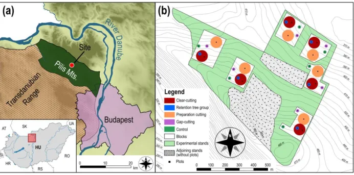
The study area 156
The study was conducted in the Pilis Mountains, Hungary (47°40′ N, 18°54′ E; Fig. 1.a) 157
using experimental plots situated on moderate (7.0–10.6°), northeast-facing slopes on a 158
broadened horst-plateau (Hosszú-hegy, 370–470 m above sea level). The climate is humid 159
continental (moderately cool–moderately wet class), the mean annual temperature is 9.0–9.5°C 160
(16.0–17.0°C during the growing season) and the mean annual precipitation is 650 mm (the total 161
summer precipitation is 350 mm) (Dövényi 2010). The bedrock consists of limestone and 162
sandstone with loess (Dövényi 2010). The soil depth varies along the slight topographic gradient 163
from 70 cm (near the ridge) to 250 cm (in the lower part of the site), although the physical and 164
chemical variables of the topsoil (the upper 50 cm) are similar in the area. Soils are slightly 165
acidic (pH of the 0–20 cm layer is 4.6 ± 0.2). The soil types are Luvisols (mainly brown forest 166
soil with clay illuviation) and Rendzic Leptosol (for further information, see Kovács et al. 2018).
167
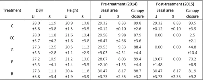
The experimental site was established in a 40 ha sized homogeneous unit of managed, 80 168
years old two-layered sessile oak–hornbeam forest stand (Natura 2000 code: 91G0; Council 169
Directive 92/43/EEC 1992) with a relatively uniform structure, homogeneous canopy closure 170
(Appendix S1: Table S1) and tree species composition as a consequence of the applied 171
shelterwood silvicultural system. The upper canopy layer (mean height: 21 m) is dominated by 172
sessile oak, the subcanopy layer is primarily formed by hornbeam (mean height: 11 m). Other 173
woody species are rare, individuals of Fraxinus ornus L., Fagus sylvatica L., Quercus cerris L., 174
and Prunus avium L. can be found as admixing tree species. Before the experimental treatments, 175
the shrub layer was scarce and mainly consisted of the regeneration of hornbeam and Fraxinus 176
ornus L. with a lower cover of shrub species (e.g., Crataegus monogyna Jacq., Cornus mas L., 177
10
Ligustrum vulgare L., and Euonymus verrucosus Scop.). The understory layer was initially 178
formed by general and mesic forest species (Carex pilosa Scop., Melica uniflora Retz., 179
Cardamine bulbifera L., Galium odoratum (L.) Scop., and Galium schultesii Vest.) and had a 180
cover of approximately 45%.
181 182
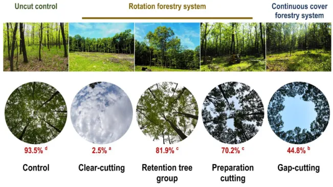
Experimental design 183
Five treatment types were implemented following a randomized complete block design in 184
six replicates (hereafter blocks) that resulted in 30 plots (Figure 1b): (1) control (C) with 185
unaltered stand characteristics; (2) clear-cutting (CC) creating 0.5 ha sized circular clear-cuts by 186
eliminating every tree individual (DBH ≥ 5 cm and/or height ≥ 2 m) within areas of 80 m in 187
diameter; (3) gap-cutting (G) represented by circular artificial gaps with approximately 1:1 gap 188
diameter/intact canopy height ratio (diameter: 20 m, area: 0.03 ha); (4) preparation cutting (P) as 189
uniform partial cutting within a circle with a diameter of 80 m (the complete subcanopy-layer, 190
and 30% of the initial total basal area of the upper canopy layer was removed in a spatially even 191
arrangement); and (5) circular retention tree group (R) within the clear-cuts where all of the tree 192
and shrub individuals were retained as a 0.03 ha sized (diameter: 20 m) circular patch of retained 193
trees. Treatments were implemented in the winter of 2014–2015. A more detailed description of 194
the experimental design and the treatments can be found in the work of Kovács et al. (2018) and 195
in the Appendix S1 (Fig. S1.).
196 197
Data collection 198
Systematic microclimate measurements were taken in the center of each plot. Temporally 199
synchronized data collection was carried out using 4-channeled Onset ‘HOBO H021-002′ data 200
11
loggers (Onset Computer Corporation, Bourne, MA, USA). In the studied years (2014–2017), 201
every month of the growing season (March–October), 72 hr logging periods were applied with 202
10 min logging intervals. Photosynthetically active radiation (PAR, λ = 400−700 nm;
203
μmol m−2 s−1) was measured at 150 cm above ground level, using Onset ‘S-LIA-M003′ quantum 204
sensors. Air temperature (Tair; °C) and relative humidity (RH, %) data were collected 130 cm 205
above ground level with Onset ‘S-THB-M002′ sensors (Onset Computer Corporation, Bourne, 206
MA, USA) housed in standard radiation shields against direct sunlight. Soil temperature (Tsoil; 207
°C) was measured with ‘S-TMB-M002′ sensors (Onset Computer Corporation, Bourne, MA, 208
USA) placed 2 cm below ground. Soil water content (SWC; m3/m3) data were collected using 209
Onset ‘S-SMD-M005′ soil moisture sensors (Onset Computer Corporation, Bourne, MA, USA) 210
buried 20 cm below ground level to measure the average soil moisture at 10–20 cm soil depth.
211
Air temperature and relative humidity data were used to calculate vapor pressure deficit (VPD;
212
kPa), which characterize the actual drying capacity of air (using the equations recommended by 213
Allen et al. 1998).
214
The collected and manually screened microclimate data were imported into a SpatiaLite 215
4.3.0a database (Furieri 2015) and were split into 24 h subsets. The experiment followed a 216
Before-After Control-Impact design (Stewart-Oaten et al. 1986): the measurement of all 217
variables started in 2014 (pre-treatment year) applying the same methodology and permanent 218
device-sets that were used in the post-harvest period (2015-2017).
219
12 Data analysis
220
For the univariate analyses, one randomly chosen 24 h microclimate dataset per month was 221
used (eight months in one growing season). For exploring the effects of treatment types, relative 222
values were calculated as differences from the control (separately in each block). Thereby, we 223
excluded the effects of the temporal differences of actual weather conditions and seasons, as well 224
as the spatial heterogeneity between the blocks. Daily mean, minimum, maximum and interquartile 225
range (IQR) of PAR, Tair, RH, VPD, Tsoil, SWC variables were computed and analyzed. As SWC is 226
a rather stationary variable within a day, only its mean was involved in the analysis. For PAR, 227
measurements between 6.00 and 18.00 (local time) were analyzed, and the daily minimum and 228
maximum values were excluded from the modelling. To investigate the effect of the treatments and 229
years on the microclimate variables, linear mixed effects models (random intercept models) with a 230
Gaussian error structure were used (Faraway, 2006). Where necessary, the response variables were 231
transformed to achieve the normality of the model residuals. The treatment (four levels: CC, G, P, 232
R), year (three levels: 2015, 2016, 2017) and their interaction were used as fixed factors, while the 233
block was specified as a random factor. The models’ goodness-of-fit values were measured by a 234
likelihood-ratio test-based coefficient of determination (R2LR; Bartoń 2016), the explanatory power 235
of the fix factors were evaluated by analysis of deviance (F-statistics; Faraway 2006). The 236
differences between the treatment levels were evaluated using Tukey’s multiple comparisons 237
procedure (alpha = 0.05) for all of the pairwise comparisons based on the estimated marginal 238
means. The significance of the differences between the control and the other treatment levels was 239
tested by linear mixed effects models without intercept (Zuur 2009). The pre-treatment data 240
(collected in the growing season of 2014) were analyzed separately following the same 241
methodological framework (Appendix S1: Table S2.).
242
13
We applied multivariate ordination methods for exploring the relative importance of the 243
microclimate variables in the separation of the treatments. Absolute diurnal datasets (mean, 244
minima, maxima and IQR of the raw microclimate data) were used during these analyses 245
because control data were also involved in these comparisons. These analyses were carried out in 246
each studied year (2014–2017) separately. Only Tair, RH, VPD, Tsoil and SWC variables were 247
used during the evaluations. PAR variables were excluded since their effect is hardly separated 248
from treatments (the applied treatments directly modified the canopy closure of the plots). The 249
separation of the plots by microclimate variables (using treatment as a priori grouping variable) 250
were explored by multivariate linear discriminant analysis (LDA; Podani 2000). We used 251
generalized microclimate data of the vegetation periods for the LDAs to exclude the effects of 252
seasonality, therefore standardized principal component analyses (PCA; Podani 2000) were 253
performed on the eight monthly measurements of each variable for all observed years separately;
254
and the first canonical axes were used to create input matrices (Appendix S1: Fig. S2.). The 255
explained variance of the first axes of these PCAs ranged between 38−88%. This approach 256
enabled to explain the highest proportion of the total variance of a given microclimate variable 257
throughout a growing season. During the four years of data collection the database contained 258
4.89% of missing values ranging 0%−20% between the months. For incomplete microclimate 259
datasets, the iterative PCA method (Ipca) suggested by Dray and Josse (2015) was performed.
260
Separation between the treatments was measured by permutational multivariate analysis of 261
variance (PERMANOVA based on Canberra metrics; Podani 2000, Anderson 2017) with 9999 262
permutations. Theseparability power of the microclimate variables among treatment levels were 263
tested by Wilks’ lambda with F-test approximation performed in multivariate analysis of 264
variance (MANOVA) for each separate year (Borcard et al. 2018).
265
14
The data analyses were performed using R version 3.4.1 (R Core Team 2017). Add-on 266
package ‘nlme’ was applied for the linear mixed effects models (Pinheiro et al. 2017), ‘lsmeans’
267
for multiple comparisons (Lenth 2016), and ‘MuMIn’ package for pseudo-R2 values (Bartoń 268
2016). PCAs were obtained by ‘vegan’ (Oksanen et al. 2018), Ipca procedures by ‘missMDA’
269
(Josse and Husson 2016), and LDAs by ‘MASS’ (Venables et al. 2002) packages.
270 271
Results 272
General treatment effects 273
The pre-treatment conditions of the plots selected for the different treatment levels were 274
similar in 2014 – although there were some differences between the plots in the case of air 275
temperature (dTair) and soil moisture (dSWC) due to the heterogeneity of the site conditions (Fig.
276
2–4., Appendix S1: Table S2).
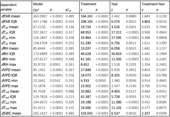
277
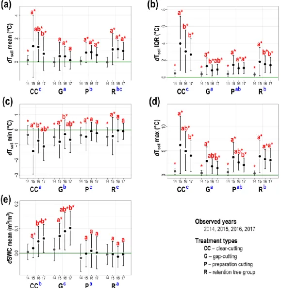
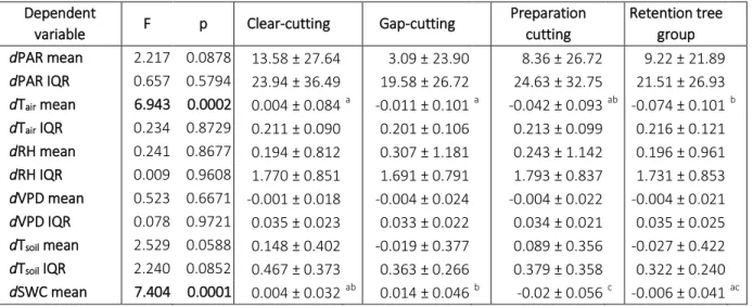
In general, we detected strong treatment effects on each examined variables (Table 1). The 278
maxima and interquartile ranges (IQRs) of the microclimate variables departed from the control 279
values in every observed year, but in some cases means and minima could remain similar to the 280
conditions measurable in the closed stands (Fig. 2–4.). For each variable, the treatment effect 281
was much more pronounced than the time effect. The strongest treatment effect was observed for 282
light variables (dPAR), dSWC and the interquartile range of dTair, air humidity (dRH) and soil 283
temperature (dTsoil) (Table 1).
284
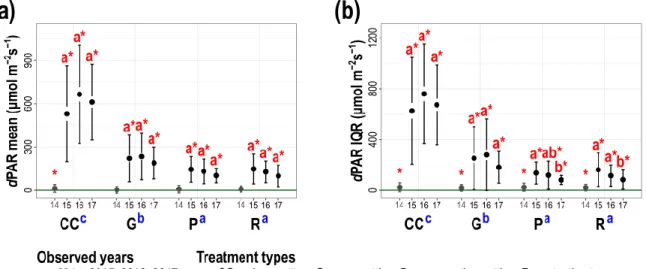
The most illuminated environment was created by clear-cutting (Fig. 2. a) with the highest 285
daily range and (Fig.2. b). Similarly, substantial increment but lower incoming radiation was 286
present in the gap-cuts (Fig.2. a). The light conditions were significantly lower and less 287
15
heterogeneous in the preparation cuts and the retention tree groups than in the prior two types, 288
but in both types, they were significantly higher than in the control.
289
The mean and the IQR of the dTair was the highest in the clear-cuts (mean ≈ 0.3°C and IQR 290
> 1°C; Fig. 3. a and b), moreover, this was the only treatment where both minima and maxima 291
were significantly different from the other treatments (Fig. 3. c and d). The mean dTair was 292
buffered the most in the preparation cuts and gap-cuts (Fig. 3. a). The variability of dTair was 293
reduced most effectively in the gap-cuts and preparation cuts, however, the latter could buffer the 294
maxima more effectively (Fig. 3. b–d). The changes in mean dTair in the retention tree groups 295
were similar to the clear-cut levels but IQRs and extrema were significantly reduced.
296
dRH means were the lowest in the retention tree groups and clear-cuts (Fig. 3. e). but in 297
clear-cuts it had higher variability and higher maximum values (Fig. 3. f–h). In the preparation 298
cuts and gap-cuts, the humidity remained similar to the control levels with the lowest variability 299
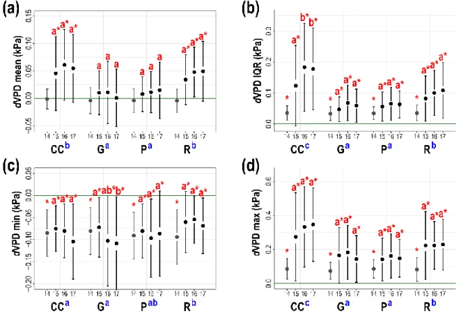
(Fig. 3. e, f). The mean of the vapor pressure deficit (dVPD) showed a similar pattern as dTair but 300
its values did not depart significantly from the control levels in the gap- and partial cuts 301
(Appendix S1: Fig. S3.).
302
In general, dTsoil differed significantly in almost every treatment from the control, the only 303
exception was the mean in gap-cutting that could preserve the levels of uncut control (Fig.4. a–
304
d). The highest dTsoil was measured in the clear-cuts and retention tree groups (approx. 1°C; Fig.
305
4. a), however, the latter treatment type induced less variable temperature (Fig. 4. b). The coolest 306
soil environment with the lowest IQR was detected in the gap-cuts. dTsoil minima were 307
significantly lower in gap- and clear-cuts than in preparation cuts and retention tree groups (Fig.
308
4. c).
309
16
The highest soil moisture was detected in gap-cuts (Fig. 4. e). dSWC was significantly 310
higher in the clear-cuts and even more in the gap-cuts than in the controls, while it remained 311
similar to the levels of the closed stands in preparation cuts and retention tree groups.
312 313
Temporal changes 314
In contrary to our expectations, in most cases there was no detectable unambiguous decrease 315
in the departures from the control levels between 2015 and 2017. The pattern of the microclimate 316
variables among the different treatment levels were relatively similar throughout the sampled 317
growing seasons, however, significant year effects were also discovered in many cases (Table 1, 318
Fig. 2–4.). The directions of these temporal changes were different and we often had unimodal 319
response: the differences from the uncut control increased from the first to the second post- 320
treatment year (from 2015 to 2016) and started to decrease between 2016 and 2017 returning to 321
the level of 2015 by 2017 (e.g., mean, IQRs and maxima of dTair, or dRH variables in most of the 322
treatments Fig. 3.). However, the differences became more pronounced in the case of dTair
323
minima (Fig. 3. a). We found that light variables decreased in preparation cuts and retention tree 324
groups during the three years, while they had a unimodal-like response in clear-cuts and gap-cuts 325
(Fig. 2.). Detectable moderating effect was present in the case of dTsoil mean, IQR and maxima, 326
mainly in case of clear-cuts and retention tree groups (Fig. 4. a, b, d), while minima had a 327
unimodal response (Fig. 4. c). Departures in dSWC enhanced over time in gap-cuts and clear- 328
cuts (Fig. 4. e).
329
Furthermore, we also detected significant seasonal effect on the responses of microclimate 330
variables: in most cases the effect sizes were the highest in the peak of the growing season (in 331
summer), which is consistent in every observed year (Appendix S1: Fig. S4.).
332
17 Separation among treatments
333
As it was hypothesized, plots did not show clear pattern before the treatments (F = 0.464, P 334
= 0.2145 according to the performed PERMANOVAs), the first canonical axis explained 52.5%
335
of the total between group variance, the second axis 22.1% (Fig. 5. a). The strongest separation 336
could be detected in 2016 (F = 4.342, P < 0.0001), with 79.4% and 10.9% of explained variance 337
by LD1 and LD2, respectively (Fig. 5. c). Separability power of the LDAs were high in 2015 338
(Fig. 5. b) and 2017 (Fig. 5.d) as well (F = 2.311, P < 0.0001 and F = 3.479, P < 0.0001, 339
respectively). However, while separation of control and clear-cutting was more pronounced and 340
the other three groups overlapped in 2016 (Fig. 5. c), all treatment types showed higher 341
separation in 2015 and 2017 (Fig. 5. b and d, respectively), although the relative partition 342
between control and clear-cutting was weaker.
343 344
The main drivers of the separation 345
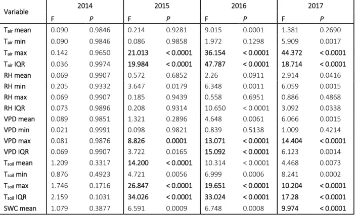
We demonstrated that if light variables are excluded, in the first three growing seasons, 346
treatment effect was mostly based on the microclimate variables that are closely related to the 347
incoming energy (Tair, VPD, Tsoil) and principally their maxima and IQRs (Table 2). During the 348
observed three years, only a slight realignment was observed. In the first year after the cuttings 349
(2015), the IQR and maximum of Tsoil was the most important variable, while in the next two 350
growing seasons, the highest F-values were related to the maximum and IQR of Tair. SWC can be 351
described as an important variable for separation only in the third growing season (2017).
352 353 354
18 Discussion
355
General treatment effects 356
As it was presumed, we could demonstrate strong and consistent treatment effects in the 357
case of the measured microclimate variables in the first three years after the silvicultural 358
interventions. Because all tree individuals were removed during clear-cutting, the most drastic 359
increase of incoming light, and consequently, the mean air and soil temperature, vapor pressure 360
deficit, and especially their variability were the highest in clear-cuts. Similarly, the extrema of 361
the variables were the most pronounced following clear-cutting. Soil water content increased 362
significantly compared to the control levels. A limited, but considerable moderating effect was 363
detected in the retention tree groups: although the means of dTair, dRH, dVPD and dTsoil were 364
similar to that in the clear-cuts, IQRs were ameliorated by these small patches of standing trees.
365
Gap-cutting could provide on the one hand an increased level of dPAR and dSWC, but on the 366
other hand artificial gaps of the size of the average tree height could maintain a buffered, cool 367
and humid environment. As with gap-cutting, preparation cutting could notably preserve the 368
closed forest conditions, without the increase of dSWC levels.
369
Light variables differed the most from the control levels because the applied treatments 370
modified the canopy closure and the spatial arrangement of the remained tree individuals first 371
and foremost (Chen et al. 1999, Heithecker and Halpern 2006, Grayson et al. 2012, Tinya et al.
372
2019). Incoming radiation was the highest and the most variable in the clear-cuts where all tree 373
individuals were harvested. Gap-cutting also created a brighter environment but PAR was 374
significantly lower than it was detected in the clear-cuts because of the smaller sky view factor 375
(Carlson and Groot 1997, Ritter et al. 2005, Kelemen et al. 2012). Insolation was lower and 376
similar to each other in the preparation cuttings and retention tree groups, although both were 377
19
significantly more illuminated than the uncut control plots in the surveyed years. Our results 378
from the preparation cuts are similar to moderate thinning and partial harvesting due to the 379
comparable harvesting processes (Weng et al. 2007, Grayson et al. 2012).
380
Air variables are primarily coupled to the incoming solar radiation. As clear-cutting created 381
the most open environment within this experimental framework, air temperature and vapor 382
pressure deficit were the highest, while air humidity was the lowest in this treatment. Many 383
studies reported substantial departures in these variables (e.g., Liechty et al. 1992, Keenan and 384
Kimmins 1993, Chen et al. 1999, Davies-Colley et al. 2000), our observations are the most 385
similar to the findings of Carlson and Groot (1997) and von Arx et al. (2012) who reported <1°C 386
increase of Tair and <5% decrease of RH averaged to the whole growing season. However, the 387
measured departures can be significantly higher in the fully-leaved period (Kovács et al. 2018).
388
Effect sizes induced by the applied silvicultural treatments presumably depend on the 389
macroclimate (especially, temperature and precipitation), topography, site conditions (e.g. soil 390
moisture) and stand type (tree species composition and structural heterogeneity mainly) 391
(Aussenac 2000; von Arx et al. 2013; Ashcroft and Gollan, 2013; De Frenne et al. 2019).
392
Nevertheless, in the case of air temperature, we found similar order of magnitude of temperature 393
offset in various European forest stands reported by Zellweger et al. (2019).
394
We demonstrated that retention tree groups in the size of one tree height can mediate the 395
thermal extremes and drying capacity of the ambient air but not their mean values which are a 396
definite aim in creating aggregated retention trees (Vanha-Majamaa and Jalonen 2001).
397
However, we found that minimum Tair remains similar in retention tree groups, gap-cuts and 398
preparation cuts.
399
20
In contrary to the clear-cutting, gap-cutting induced only moderated increase in Tair despite 400
the high amount of incoming light. Abd Latid and Blackburn (2010) demonstrated that since the 401
diffuse fraction is more pronounced in gaps, the heating is less intensive. Furthermore, RH and 402
VPD levels are similar to the humidity of ambient air in closed stands which can be addressed to 403
the evaporative cooling, the shading of the surrounding tree individuals as well as the lowered 404
lateral air mixing (Ritter et al. 2005, Muscolo et al. 2014) 405
Regarding soil temperature variables, the increased solar irradiance had an even more 406
explicit effect than it was present for air temperature values which concurs previous studies 407
(Carlson and Groot 1997, Rambo and North 2009, von Arx et al. 2013). Thus, for example 408
retention tree group could moderate the extrema of Tsoil better than Tair due to the shading 409
provided by remained overstory (Heithecker and Halpern 2006). The lowest and most stable Tsoil
410
was present in the gap-cuts due to the shading effect of the neighboring trees and the evaporative 411
cooling of the moisture content of the topsoil (Gray et al. 2002, von Arx et al. 2013). Moreover, 412
opposing previous studies (e.g., Ritter et al. 2005, Abd Latif and Blackburn 2010), soil 413
temperature remained similar to the values of the uncut control.
414
In contrary to our expectations, the most significant increase in soil moisture was observable 415
in gap-cuttings, while clear-cuttings caused significant but smaller increment in SWC. Changes 416
in soil moisture following the different treatments are typically based on the changes in elements 417
of the hydrological routine: the lower is the rate of interception and canopy evaporation, the 418
more increased the throughfall is and the more decreased the transpiration is (Wood et al. 2007, 419
Muscolo et al. 2014, Good et al. 2015). Because of the great relative importance of transpiration, 420
a higher increase in soil moisture was presumed after clear-cutting than gap-cutting (Good et al.
421
2015). The experienced smaller increase of SWC in the clear-cuts can be explained by the high 422
21
evaporation rates, the drying effects of the air-mixing due to the higher wind exposure (Keenan 423
and Kimmins 1993, Geiger et al. 1995, Bonan 2016). The effects of these processes were 424
presumably enhanced by the increasing transpiration rates of the rapidly developing herb layer 425
dominated by annual weeds (e.g., Conyza canadensis (L.) Cronquist and Erigeron annuus (L.) 426
Pers) and later, tall perennials (e.g., Calamagrostis epigeios (L.) Roth and Solidago gigantea 427
Aiton) (Tinya et al. 2019). We also found that in the retention tree groups, despite the 428
significantly higher VPD, the enhanced heat load and the transpiration of remnant tree 429
individuals, soil water content was only slightly lower than in the uncut plots.
430 431
Temporal changes following forestry treatments 432
According to our expectations, microclimate variables changed immediately after the 433
interventions and differed from the homogeneous conditions created by the closed canopy. In our 434
previous work describing the microclimate of the treatments one year after the interventions, we 435
revealed the seasonal pattern of microclimatic variables (Kovács et al. 2018). The highest 436
treatment effect was detected in the peak of the growing season due to the buffering effect of the 437
closed canopy, which was in agreement with other studies (e.g., Clinton 2003, Ma et al. 2010, 438
von Arx et al. 2012). In this study, we focused on the effects of the years only, however, the 439
seasonality effect is unambiguous not just in the first growing season but also in the second and 440
third years (Appendix S1: Fig. S4.).
441
The effects of forest management on microclimate variables could have various temporal 442
dynamics. The long-term treatment effects on forest microclimate were demonstrated for clear- 443
cuts in different forest types typically based on chronosequence studies. For example, in northern 444
hardwood forests, Dovčiak and Brown (2014) stressed that all microclimate variables differed 445
22
from forest interior in five years old regeneration stands, while daily temperature minimum 446
remained disparate for 15 years. Baker et al. (2014) demonstrated differences in the means and 447
variability of air temperature, relative humidity and VPD between various aged regenerating 448
clear-felled areas (7, 27 and 47 years since clear-cutting) and mature stands in Tasmania. In 449
general, they found that differences from mature stands in daily means can last up to 27 years 450
while diurnal variances recover in 7 years. On the contrary, the microclimatic changes in both 451
natural and artificial gaps are rather short-term comparing the effects of rotation forestry. The 452
recovery of light climate has typically exponential relationship with time since gap-creation 453
(Domke et al. 2007). Previous studies reported that approximately in the first three years, there is 454
no significant changes in the center of the gaps but there is an observable lateral growth that 455
decreases insolation near the edges (Ritter et al. 2005, Kelemen et al. 2012). It was found that in 456
gaps created by group selection, light regime became similar to the uncut mature stand in 13 457
years (Beaudet et al. 2004). Lewandowski and colleagues (2015) found differences in soil 458
temperature between gaps and uncut control that lasted seven years. However, single-tree and 459
group selections in mixed oak-pine forests did not show a temporal trend in the recovery of air 460
and soil temperature and relative humidity based on the analyzed 1–13 yrs chronosequence 461
(Brooks and Kyker-Snowman 2008).
462
Based on our models, we can conclude that the effects of treatment on microclimate variables 463
were stronger than the effect of time, differences from control among the treatment levels were 464
consistent throughout the first three years. Our results did not show a continuously fading trend of 465
the vast majority of the microclimate variables, not even in gap-cuts or preparation cuts suggested 466
by previous studies (e.g., Gray et al. 2002 or Ritter et al. 2005). The time-span of the 467
microclimatic regeneration strongly depends on species composition, forest structure and site 468
23
conditions (Aschroft and Gollan, 2013; Renaud et al. 2011; Petritan et al. 2013; Lu et al. 2015).
469
A substantial aspect of the temporal changes is the species-specific response of trees since 470
differences in leaf morphology and leaf area, canopy structure and crown plasticity can lead to 471
diverging light transmittance and lateral branch infilling of canopy gaps (Runkle 1998;
472
McCarthy 2001; Pretzsch 2014). This is relevant if we compare the more frequently studied 473
European beech and the usually understudied sessile oak, the dominant tree species of this 474
experiment. Sessile oak individuals often have smaller canopies, lower crown plasticity and 475
usually respond slower to the available space due to gap-openings compared to European beech 476
(Petritan et al. 2013). These attributes might lead to a slower falloff in altered site conditions than 477
it can be observed in for example beech-dominated stands. Certainly, the observed three growing 478
seasons are just a fraction of the required time-span typically reported (e.g., Liechty et al. 1992, 479
Dovčiak and Brown 2014, Baker et al. 2014). Similarly to the results of Liechty and colleagues 480
(1992), we did not have an unambiguous trend in the values of most variables but have between- 481
years distinctions instead during the first few years of the study. We found enhanced differences 482
from control in several cases comparing the first post-treatment year and the subsequent growing 483
seasons, but there are some variables for which the recovery process was detectable. Zheng et al.
484
(2000) also stated that the alterations following the harvests are variable-dependent but in this 485
experiment, we could demonstrate the treatment-specificity as well.
486
Gradual changes were detected in some state variables of the air near the ground – the 487
minimum air temperature decreased even more in the clear-cuts, retention tree groups and 488
preparation cuts, while minimum VPD departed more pronouncedly with time in the gap- 489
cuttings. However, the other variables did not show clear temporal pattern within this three 490
growing seasons.
491
24
However, continuous decrease was found in the case of light variability of retention tree 492
groups and partial cuts where three years may be sufficient for significant regeneration of the 493
branch structure of the remained overstory trees. Additionally, in the first post-harvest year, 494
retention tree groups were more exposed to the lateral sunlight penetration which was somewhat 495
moderated throughout the following years by the emergence of the epicormic shoots. However, 496
similarly to the mean of the incoming radiation, dPARIQR values are still significantly higher 497
than in the uncut control. The most noticeable hypothesized decrease in the differences over time 498
were present in the case of soil temperature. In the clear-cuts, both the mean, IQR and maximum 499
of the soil temperature seem to start converging continuously to the levels of control. Moreover, 500
this trend was also detected for dTsoilIQR in the retention tree groups and for maxima in the gap- 501
and preparation cuts. The recovery is presumably based on the natural regeneration of the herb 502
and shrub layer that were considerably different among the treatments (Tinya et al. 2019). Before 503
the treatments, understory vegetation was scarce and quasi-homogeneous. In the first year, the 504
cover and mean height were similar in the treatments and evolved distinctly after the cuttings.
505
The highest vegetation with the greatest total cover was present in the most illuminated 506
treatments, i.e. the clear-cuts and gaps. Understory vegetation absorbs a considerable amount of 507
incoming radiation, thus, lowers the surface temperature during daytime and it blocks the long- 508
wave radiative loss in the night ameliorating the cooling (Ritter et al. 2005, Brooks and Kyker- 509
Snowman 2008). This insulating effect was stressed primarily for bryophytes in boreal forests 510
(Bonan 1991, Nilsson and Wardle 2005), but it was also proved for understory herbs like 511
Calamagrostis canadensis (Michx.) Beauv. (Matsushima and Chang 2007). Interestingly, we 512
could capture the insulating effects of tree canopies in the case of minimum soil temperature. We 513
presume that the cooling of the topsoil due to the radiative loss might be less pronounced under 514
25
the remained individuals in the overstory layer of the retention tree groups and preparation cuts 515
than in the gap-cuts or in the clear-cuts where the sky view factor is higher (Carlson and Groot 516
1997, Blennow 1998).
517
Based on previous studies, the recovery of soil moisture was typically reported as a more 518
rapid process: it was less than five years in clear-cuts (Adams et al. 1991), in thinned stands 519
(Aussenac and Granier 1988) as well as in gaps (Gray et al. 2002, Ritter et al. 2005, 520
Lewandowski et al. 2015). Immediately after the felling, a transitory increase of soil water 521
content is present but as the vegetation is emerging and regenerating, water balance returns to the 522
pre-treatment level due to the enhanced transpiration by natural regeneration. This process is 523
necessarily faster in stands where partial cutting or gap-cutting was applied because of the 524
improved lateral growth of bordering branches, enhanced crown expansion and increased root 525
extraction from the adjacent closed stands towards the small openings. Additionally, recovery of 526
soil microclimate in gaps can be faster in broadleaved stands than in forests dominated by 527
coniferous species (Lindo and Visser 2003). However, we found an opposing response: the clear- 528
and gap-cutting were followed by a steady increase in the departures from the uncut control level 529
despite the regenerating herb layer. Liechty et al. (1992) reported similar processes when they 530
examined the recovery of soil moisture content in five-year-old clear-cuts created in temperate 531
hardwood forests.
532
As Davis et al. (2018) and Liechty et al. (1992) underlined, most studies focusing on the 533
temporal changes of the microclimate variables in woodlands or the buffering capacity of forest 534
canopies are often based on datasets from short term (typically 1–3 yrs) investigations.
535
Considering that the processes may be under the way, we continue the systematic measurements 536
26
(applying the same protocol) in the framework of this long-term experiment to follow up the 537
microclimatic recovery.
538 539
Separation of silvicultural treatments based on microclimatic variables 540
Beside analyzing the treatment effects on microclimate variables, we aimed to identify those 541
variables which are accountable for the possible changes in the local environment after the 542
interventions. We presumed that by unfolding the effects of treatments, we could get a more 543
complete picture about the microclimatic processes in treated forest sites, thus, better 544
conservational implications could be emerged (De Frenne et al. 2013).
545
As in the case of the temporal analyses, after a more or less homogeneous pre-treatment 546
state, the greatest separation was expected in the first post-treatment year (2015), because the 547
highest treatment effect could be presumed right after the interventions when modified canopy 548
closure is the most explicit and the effects of the regeneration of the understory as well as lateral 549
growth of the canopy are negligible, which could influence both thermal (shading and insulating) 550
and humidity conditions (via transpiration). This initial phase should be followed by a 551
homogenization as the sites recover, the natural regeneration develop and the canopy closure 552
evolve. However, the greatest separation was observed in the second year after the harvests. We 553
detected two different phenomena according to the observational years: (i) the greatest overall 554
separation in 2016 was congruent with the greatest divergence between the uncut control and 555
clear-cutting, while the other treatments pooled and overlapped; (ii) in the adjoining two years, 556
the between-group separation was more pronounced and even. These could be addressed to the 557
masking effect of the extremely modified environment followed by the clear-cutting.
558
We found that the applied treatments separated among the temperature (Tair and Tsoil) and 559
VPD maxima and their interquartile ranges and the roles of the individual variables in the 560
27
treatment effect were more or less consistent throughout the years. As it was presumed, soil 561
temperature was the most important determinant in the first year after the interventions, but in 562
the following years, the relative importance of air temperature increased. Surprisingly, soil 563
moisture became a significant determinant only in the third year in spite of the rather strong 564
treatment effect – especially in the gap-cuts and clear-cuts.
565
With the performed multivariate analyses, we can also demonstrate the reduced buffering 566
ability of the forest canopy and stand structure as a frequently stressed consequence of forest 567
management (Chen et al. 1999, Heithecker and Halpern 2006, Ewers and Banks-Leite 2013, De 568
Frenne et al. 2013, Hardwick et al. 2015). The microclimatic buffering capacity of the canopy 569
and even pronouncedly, variables related to forest structure are typically more noticeable 570
regarding the thermal maxima and the minima than the means (Liechty et al. 1992, 571
Vanwalleghem and Meentemeyer 2009, Ewers and Banks-Leite 2013, Frey et al. 2016, De 572
Frenne et al. 2019). In closed stands with different structural complexity, Frey et al. (2016) found 573
that maximum temperatures in old-growth stands could be more ameliorated than minimum 574
values (-2,5 °C and +0,7 °C, respectively). Greiser et al. (2018) observed comparable differences 575
in the effect size of the summer temperature extremes in central Sweden: the detected maximum 576
temperatures decreased by 12 °C, while minima increased by 4 °C. In congruence with these, 577
paired (forest–non-forest) studies reported similar trends: larger differences in temperature 578
maxima than in minima as well as in VPDmax than in VPDmin extremes (e.g., Chen and Franklin 579
1997, Vanwalleghem and Meentemeyer 2009, Renaud et al. 2011, von Arx et al. 2013, Davis et 580
al. 2018). Based on our results and in line with the literature compiled, it can be stated that forest 581
canopy performs its buffering capacity more on the maxima than on the minima of microclimatic 582
variables. We can suppose that through the reflectance and absorption of shortwave radiation 583
28
within the active layer of the canopy and through the shading of the understory is more effective 584
than the capturing and reflectance of longwave radiation from the soil.
585
The results of the multivariate analyses underpin that, as it has been argued in the recent 586
years, not the means of the microclimatic conditions, but rather the extrema are the most 587
influential factors shaping biological processes and ecological interactions (Suggitt et al. 2011, 588
Thompson et al. 2013, Bramer et al. 2018). Moreover, according to our results, it seems that the 589
applied forestry treatments can differently enhance the changes in the set of variables modifying 590
local climates.
591
592
Conclusions and perspectives 593
Based on the measurements performed in the first three years after the forestry treatments, 594
we can conclude that (i) the effect sizes among treatment levels were consistent throughout the 595
first three years; (ii) the climatic recovery time for variables appears to be far more than three 596
years – except for soil temperature – in all treatments and (iii) the applied silvicultural methods 597
diverged mainly among the temperature maxima. The most drastic changes were observed in 598
clear-cuts where retention tree groups could impinge only a limited buffering effect (on the 599
variability and extrema, though not on the mean). However, a relatively large gap size (one tree 600
height/gap diameter ratio) could provide a reasonably stable and humid but more illuminated 601
environment. Preparation cutting changed the forest environment only to a lesser degree.
602
Our results suggest that in mesic broadleaved forests, forestry treatments induce long-lasting 603
changes in microclimate near the ground that substantially alters the environmental conditions.
604
These changes may cause the promptly occurring alterations in communities of the forest- 605
dwelling species – which were shown for different taxa in the framework of this experiment – 606
especially in the case of organisms groups with limited movement ability (Elek et al. 2018, Tinya 607
29
et al. 2019, Boros et al. 2019). Due to the high probability of extreme thermal events, clear- 608
cutting enhances the frost damage, the heat stress as well as higher exposure of draught causing 609
local extinctions and significant compositional shifts. Moreover, from a broader prospect, 610
management types causing considerable canopy-openness on large areas, independently of the 611
characteristics (i.e. aggregated or dispersed), may precipitate the effects of climate change in 612
forested landscapes.
613
We can conclude that in managed temperate broadleaved forests (like in this study, in oak–
614
hornbeam stands), for biodiversity conservation purposes, small-scale or spatially dispersed 615
forestry treatments are desired. By applying actions belonging to continuous cover forestry (e.g., 616
gap-cutting, irregular shelterwood system), the original characteristics of the forest environment 617
can be preserved.
618 619
30 Acknowledgements
620
This research was funded by the Hungarian Scientific Research Fund (OTKA K111887), the 621
National Research, Development and Innovation Fund of Hungary (GINOP-2.3.2-15-2016- 622
00019, K128441), the Infrastructure Grant andthe “Ecology for Society Project” of Hungarian 623
Academy of Sciences (MTA KEP). B. K. was supported by the ÚNKP-17-3 New National 624
Excellence Program of the Ministry of Human Capacities. F.T. was supported by the MTA 625
Postdoctoral Fellowship Programme (PD-009/2017) and by the National Research, Development 626
and Innovation Fund of Hungary (PD 123811).
627
The study site is legally protected; the experiment was approved by the Pest County 628
Administration (permission number: KTF 30362-3/2014).
629
We are grateful for the cooperation and the joint efforts of the Pilisi Parkerdő Ltd., especially to 630
Péter Csépányi, Viktor Farkas, Gábor Szenthe, and László Simon. The authors are thankful to 631
Kristóf Kelemen for help in the database design and development and Beáta Biri-Kovács for 632
editing the manuscript. Erika Guba played an essential role in the fieldwork in 2014–2015. We 633
also thank the two anonymous Reviewers whose suggestions substantially improved the 634
manuscript.
635 636
Author’s contributions 637
The experiment was planned by P. Ó.; P.Ó. and B. K. conceived the ideas and designed the 638
methodology for the study; fieldwork was organized and performed by B. K., Cs. N. and F.T.;
639
statistical analyses were performed by B. K.; and the manuscript was written by B. K. and P. Ó.
640
with the approval of F.T. and Cs. N.
641 642