Mathematical models for balancing tasks on a see-saw with reaction time delay
Gergely Buza∗,Tamas Insperger∗
∗Department of Applied Mechanics, Budapest University of Technology and Economics and MTA-BME Lend¨ulet Human Balancing Research
Group, Budapest, Hungary (e-mail: buza1gergely@gmail.com, insperger@mm.bme.hu)
Abstract:Mechanical models of balancing a ball rolling on a see-saw (“ball and beam” system) and balancing an inverted pendulum attached to a cart rolling on a see-saw (“pendulum- cart and beam” system) are analyzed. A delayed proportional-derivative controller is modeled with four different actuation schemes. The angular position, the angular velocity, the angular acceleration of the see-saw and the torque acting on the see-saw are considered to be the variables manipulated by the control system. The corresponding mathematical models take the form of retarded, neutral and advanced functional differential equations. Stabilizability analysis shows that the ball and beam system can only be stabilized in the presence of feedback delay if the manipulated variable is the angular position of the see-saw or the torque acting on the see-saw.
The pendulum-cart and beam system can only be stabilized in the presence of feedback delay if the manipulated variable is the torque acting on the see-saw.
Keywords:ball and beam, inverted pendulum, feedback delay, stability, stabilizability.
1. INTRODUCTION
Stabilization of systems around their unstable equilibria by means of feedback control is a common task in many branches of modern sciences. Engineering structures are often operated around an unstable position for the simple cause that it is more efficient to initiate and perform sudden motions from these positions. The corresponding control process typically involves a feedback delay, which is originated from signal processing, information trans- mission and actuation lags. Many human activities can be associated with a similar feedback mechanism, one might think of simple quiet standing, gait or running where the feedback delay is the reaction time. Human balancing tasks, such as stick balancing on a fingertip or on a pingpong racket Cabrera and Milton (2002); Mehta and Schaal (2002); Milton et al. (2016); Yoshikawa et al.
(2016), quiet standing Maurer and Peterka (2005); Suzuki et al. (2012); Hwang et al. (2016), standing on pinned or rolling balance boards Chagdes et al. (2016); Molnar et al. (2017), are therefore often analyzed via simplified mechanical and mathematical models.
In this paper, two balancing tasks are investigated: (1) balancing a rolling ball on a see-saw; and (2) balancing a pendulum-cart system on a see-saw. Different control actuation concepts are modeled with and without feedback delay, which gives different types of governing equations, namely, retarded functional differential equation (RFDE), neutral functional differential equation (NFDE) and ad- vanced functional differential equations (AFDEs). The different models are compared with respect to their sta- bilizability properties.
2. MECHANICAL MODELS
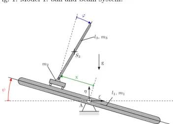
Mechanical models of balancing a ball rolling on a see- saw, also called ball and beam system and balancing an inverted pendulum attached to a cart rolling on a see-saw, called pendulum-cart and ball system are shown in Figs. 1 and 2. The ball and beam system (model 1) is a two DoF system with positionxof the ball and angleψof the see- saw being the general coordinates. The pendulum-cart and ball system (model 2) is a three DoF system with general coordinatesx,ψand angleϕof the pendulum.
Four different actuating concepts are distinguished, when the manipulated variables are:
(1) the angular position of the see-saw:ψ;
(2) the angular velocity of the see-saw: ˙ψ=ω;
(3) the angular acceleration of the see-saw: ¨ψ=ε;
(4) the torque acting on the see-saw:Q.
The output is assumed to be fed back via a PD controller in all cases. Furthermore, two more cases are distinguished based on the argument of the feedback variables:
(1) real-time continuous measurement, when x(t), ψ(t) andϕ(t) are directly fed back;
(2) continuous measurement with feedback delay, when the delayed states x(t−τ), ψ(t −τ) and ϕ(t−τ) show up in the control law.
Different models are named by combining the above no- tations. For instance, model 1.4.2 refers to model 1, with the torque being the manipulated variable, and with the feedback delay taken into account. These cases give overall 2×4×2 = 16 different models.
14th IFAC Workshop on Time Delay Systems, Budapest, Hungary, June 28-30, 2018.
ψ
x m2 g
η ξ A
l1,m1
Fig. 1. Model 1: ball and beam system.
ψ
x m2 g
ϕ
η ξ A S3
l3,m3
l1,m1
Fig. 2. Model 2: pendulum-cart and beam system.
3. MODELS FOR BALL AND BEAM SYSTEM The control concepts presented in the previous section are discussed along with a brief description of the correspond- ing stability properties.
3.1 Model 1.1
In this case, the angular position ψ of the see-saw is assumed to be manipulated by the control system based on the observation, that most human subjects solve this balancing task by simply holding the see-saw in a steady position relying on the gravity to roll the ball to the desired middle position. In this case, the mechanical model is reduced to a one DoF system and the corresponding linearized equation of motion reads
¨
x(t) =−gψ(t). (1)
Different control concepts are detailed below.
Model 1.1.1 It is assumed that the position of the rolling ball on the see-saw is measured continuously in real-time.
Equation (1) holds, and the PD control realizes ψ(t) = Pxx(t) +Dxx(t), which implies the governing equation˙
¨
x(t) +gDxx(t) +˙ gPxx(t) = 0, (2) wherePxandDxare the proportional and derivative gains.
The system is asymptotically stable ifPx>0 andDx>0.
Model 1.1.2 Here, the feedback delay τ is taken into account. Equation (1) still holds, the only difference shows up in the delayed arguments. The governing equation reads
¨
x(t) +gDxx(t˙ −τ) +gPxx(t−τ) = 0. (3)
Using the D-subdivision method, the D-curves of this system can be given as
ω= 0 : Px= 0, Dx∈R, (4)
ω >0 : Px= ω2
g cos(ωτ), Dx=ω
g sin(ωτ), (5) and the corresponding stability diagram can be seen in Fig. 3. Note that this system can be stabilized for allτ ≥0, which means that model 1.1.2 isdelay-independently stable (see Michiels and Niculescu (2007)).
Fig. 3. The stable domain and the number of unstable poles for model 1.1.2 withτ= 1s.
3.2 Model 1.2
This model is based on the assumption that the manip- ulated variable is the angular velocity of the see-saw.
The linearized equation of motion can be obtained after differentiating (1) with respect to time:
...x(t) =−gψ(t) =˙ −gω(t). (6) Model 1.2.1 For the case of real-time measurement the control can be written in the form of ω(t) = Pxx(t) + Dxx(t), thus, the governing equation reads˙
...x(t) +gDxx(t) +˙ gPxx(t) = 0. (7) The stability chart and the number of unstable poles for different parameter regions are shown in Fig. 4.
Fig. 4. Transition curves and the number of unstable poles for model 1.2.1. On lineDx>0,Px= 0 all the three characteristic roots are 0.
Model 1.2.2 In case of delayed feedback, the system is governed by
...x(t) +gDxx(t˙ −τ) +gPxx(t−τ) = 0. (8) The D-curves can be given in the form
ω= 0 : Px= 0, Dx∈R, (9)
ω >0 : Px=−ω3
g sin(ωτ), Dx=ω2
g cos(ωτ), (10) and the stability diagram can be seen in Fig. 5 forτ = 1s.
As seen in Fig. 4 and Fig. 5, model 1.2 cannot be stabilized.
Fig. 5. Transition curves and the number of unstable poles for model 1.2.2 withτ = 1s.
3.3 Model 1.3
Here, it is assumed that the manipulated variable is the angular acceleration of the see-saw. The linearized equation of motion can be obtained by taking the second derivative of (1):
x(iv)(t) =−gψ(t) =¨ −gε(t). (11) Model 1.3.1 The control of the angular acceleration takes the form ε(t) = Pxx(t) +Dxx(t) in the real-time˙ model, which, after substituted into (11), leaves us with
x(iv)(t) +gDxx(t) +˙ gPxx(t) = 0. (12) The corresponding stability diagram is shown in Fig. 6.
Note that the characteristic equation evaluated at point (Px, Dx) = (0,0) is λ4 = 0, which results in 0 being a quadruple root.
Fig. 6. Transition curves and the number of unstable poles for model 1.3.1.
Model 1.3.2 The case of delayed feedback implies x(iv)(t) +gDxx(t˙ −τ) +gPxx(t−τ) = 0. (13) The corresponding D-curves are
ω= 0 : Px= 0, Dx∈R, (14)
ω >0 : Px=−ω4
g cos(ωτ), Dx=−ω3
g sin(ωτ). (15) The stability properties of the model are shown in Fig. 7.
Asymptotic stability cannot be achieved in this case.
Fig. 7. Transition curves and the number of unstable poles for model 1.3.2 withτ = 1s.
3.4 Model 1.4
In this model, the system is assumed to be manipulated by a control torque acting on the see-saw. The corresponding 2 DoF system is governed by
m2 0 0 θ1
¨ q(t) +
0 m2g m2g 0
q(t) =
0
−Q(t)
, (16) whereq(t) = (x(t), ψ(t))T,θ1=m1l21/12 is the moment of inertia of the see-saw and Q(t) is the torque specified by the PD controller. The parameters of the model are m1 = 2kg, m2 = 1kg, l1 = 2m (see Fig. 1). Note that models 1.1, 1.2 and 1.3 were independent of these physical parameters.
Model 1.4.1 In the case of real-time output measurement (16) holds, and the control torque is given in the form
Q(t) =Pxx(t) +Dxx(t) +˙ Pψψ(t) +Dψψ(t).˙ (17) The stable domains for model 1.4.1 are given after substi- tution and the application of the D-subdivision method, and are shown in Fig. 8.
Fig. 8. Stability charts and the number of unstable poles for model 1.4.1.
Model 1.4.2 In the delayed case the control torque reads Q(t) =Pxx(t−τ) +Dxx(t˙ −τ) +Pψψ(t−τ) +Dψψ(t˙ −τ).
(18) The D-curves can be written in the form
ω= 0 : Px=−gm2, Dx∈R, (19) ω >0 : Px= cos(ωτ)
g θ1ω4−m2g2
−Pψ
ω2 g , (20) Dx= sin(ωτ)
gω θ1ω4−m2g2
−Dψ
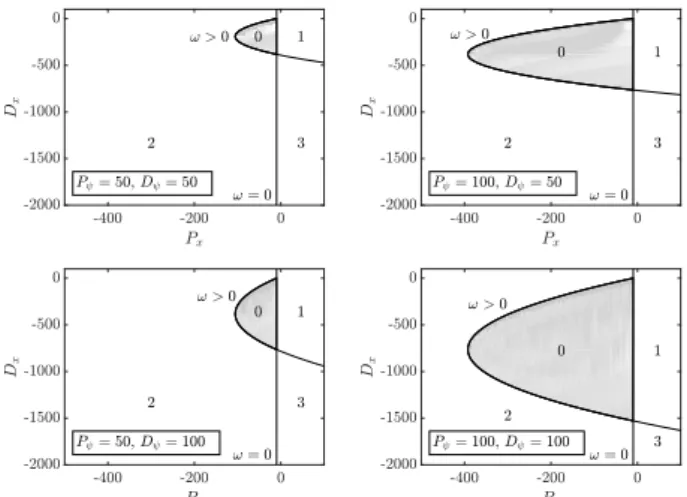
ω2 g . (21) Numerical analysis shows that the system can only be stabilized for delays less thanτcrit = 0.32s. Some sample stability diagrams for model 1.4.2 can be seen in Fig. 9.
4. PENDULUM-CART AND BEAM SYSTEM The control concepts presented in the previous section are repeated here for the pendulum-cart model rolling on the see-saw.
Fig. 9. Stable domains for model 1.4.2, withτ = 0.08s.
4.1 Model 2.1
The three-DoF mechanical model (see Fig. 2) is to be discussed from now on with the angular positionψ of the see-saw being the manipulated variable for models 2.1.×.
The linearized equation of motion takes the form ( x(t) =¨ aϕ(t)−gψ(t),
¨
ϕ(t) =bϕ(t)−ψ(t),¨
(22) where
a= 3m3g m3+ 4m2
, b= 6g(m2+m3) l3(m3+ 4m2),
with m3 = 0.1kg and l3 = 1m. The other parameters are the same as in model 1.
Model 2.1.1 Here, the control angular position reads ψ(t) =Pxx(t) +Dxx(t) +˙ Pϕϕ(t) +Dϕϕ(t),˙ (23) which, after substituted into (22), provides the correspond- ing governing equation for this model. The stability dia- gram is shown in Fig. 10.
Fig. 10. Transition curves and the number of unstable poles for model 2.1.1.
Model 2.1.2 For delayed feedback, we have
ψ(t) =Pxx(t−τ) +Dxx(t˙ −τ) +Pϕϕ(t−τ) +Dϕϕ(t˙ −τ).
(24)
The corresponding characteristic equation reads
D(λ) =Dϕλ5e−λτ+(Pϕe−λτ+1)λ4+(a+g)Dxλ3e−λτ+ +
(a+g)Pxe−λτ−b
λ2−bgDxλe−λτ−bgPxe−λτ = 0.
(25) As seen in (25) the highest derivative appears with a delayed argument, thus system (22) with (24) becomes an AFDE in this model. Consequently, model 2.1.2 is always unstable with infinitely many unstable characteristic roots.
4.2 Model 2.2
The angular velocity is assumed to be manipulated by the control system and the linearized equation of motion reads
( ...
x(t) =aϕ(t)˙ −gω(t),
¨
ϕ(t) =bϕ(t)−ω(t).˙
(26)
Model 2.2.1 In the case of real-time output measure- ment, the manipulated angular velocity takes the form
ω(t) = ˙ψ(t) =Pxx(t) +Dxx(t) +˙ Pϕϕ(t) +Dϕϕ(t).˙ (27) The stability chart for this model can be seen in Fig. 11.
Fig. 11. Stability boundaries and the number of unstable poles for model 2.2.1.
Model 2.2.2 With feedback delay, the control input takes form
ω(t) =Pxx(t−τ) +Dxx(t˙ −τ) +Pϕϕ(t−τ) +Dϕϕ(t˙ −τ).
(28) Equation (26) with (28) gives a NFDE. The corresponding characteristic equation reads
D(λ) = (1 +Dϕe−λτ)λ5+Pϕλ4e−λτ−
−bλ3+
(a+g)λ2−bg
(Px+λDx)e−λτ = 0. (29) Note that, according to the strong stability criteria, (29) has infinitely many unstable roots if |Dϕ| >1. However, it can be shown that the system is still unstable for any control parameters and delays even if |Dϕ| < 1. Some corresponding stability charts are shown in Fig. 12.
4.3 Model 2.3
This model discusses the case where the angular acceler- ation is assumed to be manipulated by the controller in
Fig. 12. Transition curves and the number of unstable poles for model 2.2.2 withτ= 0.01s.
the three-DoF system. The linearized equation of motion reads
( x(iv)(t) =aϕ(t)¨ −gε(t),
¨
ϕ(t) =bϕ(t)−ε(t).
(30) System (30) fails Kalman’s criteria of controllability, thus both model 2.3.1 and 2.3.2 are not controllable by means of angular acceleration control, therefore they are not discussed here further.
4.4 Model 2.4
In this model, a torque type control is assumed. Since the angular position is not restricted by the control system, the corresponding model has three degrees of freedom. The linearized equation of motion reads
M¨q(t) +Sq(t) =Q∗(t), (31) where q = (x(t), ψ(t), ϕ(t))T, Q∗(t) = (0,−Q(t),0)T and
M=
m2+m3 −l3m3
2 −l3m3
2
−l3m3
2 1
12(l21m1+ 4l23m3) l23m3
3
−l3m3
2
l23m3
3
l23m3
3
, (32)
S=
0 g(m2+m3) 0 g(m2+m3) −1
2gl3m3 −1 2gl3m3
0 −1
2gl3m3 −1 2gl3m3
. (33)
Model 2.4.1 The control torqueQ(t) takes the form Q(t) =Pxx(t) +Dxx(t) +˙ Pψψ(t)+
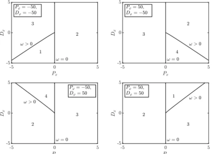
+Dψψ(t) +˙ Pϕϕ(t) +Dϕϕ(t).˙ (34) Some sample stability charts are shown in Fig. 13.
Model 2.4.2 For delayed feedback, the control torque is Q(t) =Pxx(t−τ) +Dxx(t˙ −τ) +Pψψ(t−τ)+
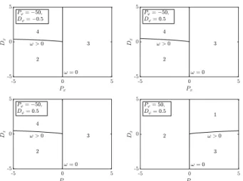
+Dψψ(t˙ −τ) +Pϕϕ(t−τ) +Dϕϕ(t˙ −τ). (35) Some stability diagrams for model 2.4.2 can be seen in Fig. 14 forτ= 0.01s. The critical delay, where the system cannot by stabilized any more, was found numerically to be τcrit≈0.05s.
Fig. 13. Stable domains for model 2.4.1.
Fig. 14. Stable domains for model 2.4.2 withτ= 0.01s.
5. RESULTS
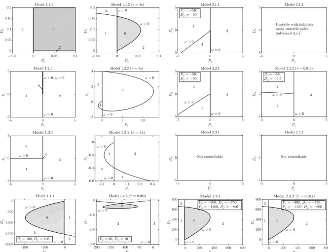
An overview on the stabilizability properties of the differ- ent models are presented in Fig. 15. While the ball and beam system (model 1) can be stabilized via the angular position of the see-saw and via a control torque acting on the see saw, the the pendulum-cart and beam system (model 2) can only be stabilized via a control torque. The ball and beam system can be stabilized via the angular position of the see-saw independently on the value of the feedback delay. In case of stabilization via control torque, there is a critical delay, which limits stabilizability. For model 1, the critical delay is τcrit = 0.32s, for model 2, it is τcrit = 0.05s. This analysis confirmed the intu- itive assumption that it is more difficult to stabilize the pendulum-cart and beam system than the ball and beam system.
An experimental device was built for each mechanical model in order to perform balancing tasks by human subjects. The typical human reaction time in visual tasks is around 200∼250ms Milton et al. (2016), which implies that for humans it is impossible to balance the pendulum- cart and beam system. Balancing trials by 12 subjects confirmed this assumption. None of 12 subjects were able to keep the pendulum in the upright position for more than a second for the pendulum-cart and beam system, while all of them were able to drive the ball to the desired middle
Fig. 15. Sample stability charts for the different models. Only models 1.1.×, 1.4.×and 2.4.×can be stabilized.
position for the ball and beam system within 10 ∼ 15 seconds. These analysis supports that the human either manipulates the angular position ψ of the see-saw or applies a control torque on the see-saw during the ball and beam balancing task. The only possible way to balance the pendulum-cart and beam system is the application of a control torque on the see-saw, but, for the presented parameter regions, this process can be stable only if the feedback delay is much shorter than the typical human reaction time, namely, less than 0.05s.
ACKNOWLEDGEMENTS
The research reported in this paper was supported by the Higher Education Excellence Program of the Ministry of Human Capacities in the frame of Biotechnology research area of Budapest University of Technology and Economics (BME FIKP-BIO).
REFERENCES
Cabrera, J.L. and Milton, J.G. (2002). On-off intermit- tency in a human balancing task. Physical Revies Let- ters, 89, 158702.
Chagdes, J.R., Rietdyk, S., Haddad, J.M., Zelaznik, H.N., Cinelli, M.E., Denomme, L.T., Powers, K.C., and Ra- man, A. (2016). Limit cycle oscillations in standing human posture. J. of Biomechanics, 49, 1170–1179.
Hwang, S., Agada, P., Kiemel, T., and Jeka, J.J. (2016).
Identification of the unstable human postural control system. Frontiers in Systems Neuroscience, 10, 22.
Maurer, C. and Peterka, R.J. (2005). A new interpretation of spontaneous sway measures based on a simple model of human postural control. Journal of Neurophysiology, 93, 189–200.
Mehta, B. and Schaal, S. (2002). Forward models in visuomotor control. Journal of Neurophysiology, 88, 942–953.
Michiels, W. and Niculescu, S.I. (2007). Stability and Stabilization of Time-Delay Systems (Advances in De- sign and Control). Society for Industrial and Applied Mathematics, Philadelphia, PA, USA.
Milton, J., Meyer, R., Zhvanetsky, M., Ridge, S., and In- sperger, T. (2016). Control at stabilitys edge minimizes energetic costs: expert stick balancing. Journal of the Royal Society Interface, 13, 20160212.
Molnar, C.A., Zelei, A., and Insperger, T. (2017). Estima- tion of human reaction time delay during balancing on balance board. InProceedings of 13th IASTED Interna- tional Conference on Biomedical Engineering (BioMed), 195.
Suzuki, Y., Nomura, T., Casadio, M., and Morasso, P.
(2012). Intermittent control with ankle, hip, and mixed strategies during quiet standing: A theoretical proposal based on a double inverted pendulum model. Journal of Theoretical Biology, 310, 55–79.
Yoshikawa, N., Suzuki, Y., Kiyono, K., and Nomura, T. (2016). Intermittent feedback-control strategy for stabilizing inverted pendulumon manually controlled cart as analogy to human stick balancing. Frontiers in Computational Neuroscience, 10, 39.