Human balancing on rolling balance board in the frontal plane
Csenge A. Molnar∗ Ambrus Zelei∗ Tamas Insperger∗
∗Department of Applied Mechanics, Budapest University of Technology and Economics and MTA-BME Lend¨ulet Human Balancing Research
Group, (e-mail: csenge.molnar@mm.bme.hu, zelei@mm.bme.hu, insperger@mm.bme.hu).
Abstract:Human balancing on rolling balance board in the frontal plane is analyzed using a two DoF mechanical model, where the human body is modeled by a four-bar linkage mechanism and the geometry of the balance board can be adjusted. Human nervous system is assumed to employ a proportional-derivative controller with constant feedback delay identical to the human reaction time. It is shown that a critical feedback delay exists for each geometry of the balance board. If the reaction delay is larger than the critical one, then there are no stabilizing control gains. A numerical algorithm was developed in order to find the critical time delay based on the mechanical model. The numerical results are compared with real balancing trials, and the corresponding feedback delays in the model are compared to the results of actual reaction time tests.
Keywords:balance board, human balancing, reaction delay, stability, stabilizability 1. INTRODUCTION
Analysis of human balancing while standing still or walk- ing is becoming more and more important nowadays be- cause many accidents can be connected falls due to the loss of balance, especially among the elderly. In addition, theo- retical and experimental investigation of human balancing facilitates to understand the control concept employed by the human nervous system. From mechanical point of view, human standing still is the stabilization of the human body around an unstable equilibrium. Sensory organs perceive information about the position of the body, this informa- tion is processed by the brain, and signals are delivered to the musculature, which result in a corrective movement.
This feedback mechanism requires certain amount of time, which is often referred to as reaction time. One of the most important and commonly encountered problems of human balancing is how our brain processes the information de- livered by the sensory organs and how it determines the instruction sent to the muscles.
Mechanical models for standing still in the sagittal plane typically involve a pinned inverted pendulum model sub- ject to a delayed feedback, see, e.g., Maurer and Peterka (2005); Milton et al. (2009); Stepan (2009); Suzuki et al.
(2012); Hwang et al. (2016). Models for standing still in the frontal plane are usually based on a four-bar linkage mech- anism, see, e.g., Goodworth and Peterka (2010); Bingham et al. (2011); Hajdu et al. (2016). In these models, most of the mechanical parameters, such as mass, inertia, stiffness, are related to the human body, whose estimation involves many uncertainties. When human subjects are balancing on (pinned or rolling) balance board, then the mechanical properties of the balance board can easily be measured, and can be introduced into the mechanical model (see Chagdes et al. (2016); Molnar et al. (2017)). Furthermore,
the parameters of the balance board can be adjusted, thus the balancing performance at different conditions can be investigated this way.
Balancing on a rolling balance board in the sagittal plane was investigated in Molnar et al. (2017). In this paper, balancing on the same balance board in the frontal plane is analyzed. The corresponding model is an extension of the four-bar linkage models for standing still in the frontal plane. The main goal of the paper is to compare the mechanical model with experimental observations in terms of the reaction delay.
2. MECHANICAL MODEL 2.1 Introduction of the model
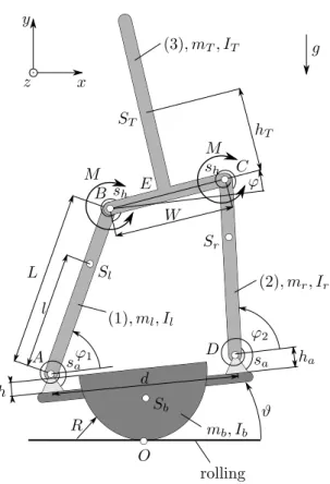
Balancing on a rolling balance board in the frontal plane (x, y) is modeled by a two-degree-of-freedom system shown in Fig. 1. The human body in the frontal plane is modeled as a four-bar linkage mechanism based on the model by Bingham et al. (2011). The two legs are modeled as two homogeneous rigid bars, which are connected to the upper (T-shaped) body by ideal pins. The balance board is assumed to roll on the ground. The generalized coordinates are chosen to be the angle ϕ of the trunk relative to the balance board and the angular displacement ϑof the balance board relative to the environment. The feet are considered to be fixed to the balance board and it is assumed that the ankle behaves as a pin between the legs and the balance board (see pointsAandD in Fig. 1).
It is assumed that the human brain controls by signals proportional to the angular offset and velocity of the human body and the balance board. Therefore the control process is modeled as a delayed PD controller with a
14th IFAC Workshop on Time Delay Systems, Budapest, Hungary, June 28-30, 2018.
d
A D
C B
l
L Sl
ST
Sr
E
ϕ1
ϕ2 ϕ
hT
W
ϑ (3), mT, IT
(2), mr, Ir
(1), ml, Il
Sb
O
rolling
ha
h
R x y
z
g
M
M sh
sh
sa sa
mb, Ib
Fig. 1. Two DoF mechanical model.
constant time delay τ, which describes the reaction time of the balancing subject. It is assumed that the control torque is acting between the hip and the legs at pointsB and C in Fig. 1. Passive stiffness at the ankles and the hip are determined according to the literature, while the passive damping at these joints are neglected. The ankle stiffness is estimated using
sa = 0.91mgl
4, (1)
which was determined for quiet standing in sagittal plane by Loram and Lakie (2002). Stiffness of the hip can be approximated using hip angle-moment curves (see Winter et al. (1998), Yoon and Mansour (1982), Riener and Edrich (1999), A. Silder and Thelen (2007)). Here, the curve of Riener and Edrich (1999) was used to get the approximate valuesh≈17 Nm/rad for the torsional stiffness of the hip.
2.2 Balance board
The balance board is shown in Fig. 2. The adjustable parameters are the radiusRof the wheels and the distance hof the board measured from the center of the wheel. The wheels were manufactured with radii of 2.5, 5, 7.5, 10, 12.5, 15, 20 and 25 cm and the distance hcan be changed by steps of 2.5 cm for each wheel. Thickness of the plywood was 21 mm, and its density was 700 kg/m3. Note that some of the wheels were manufactured with raised edge, therefore board distancehcan take negative value.
The center of gravity, mass, and mass moment of inertia of the balance board was calculated using the geometry and the mass of the board elements. The feet was assumed to move together with the board, therefore its mass and
Fig. 2. Balance board.
inertia was added to the mass and inertia of the balance board.
2.3 Balancing subjects
The parameters of the human body segments were deter- mined based on the data in de Leva (1996). The upper part of the human body is considered as a rigid body, which includes the head, the trunk, the upper arms, the forearms and the hands. The leg is constructed by the thigh and the shank. The masses of bodies (1), (2), and (3) in Fig. 1 are calculated as the sum of the corresponding segments. The length of each segment were estimated from the height of the balancing subject. Table 1 summarizes the data, which were measured for each balancing subject.
Using these parameters, the center of gravity, mass and mass moment of inertia of bodies (1), (2) and (3) in Fig. 1 can be estimated.
Table 1. Parameters of balancing subjects.
Notation S1 S2 S3 S4
ha 0.07 [m] 0.08 [m] 0.085 [m] 0.11 [m]
W 0.28 [m] 0.27 [m] 0.27 [m] 0.33 [m]
d 0.35 [m] 0.32 [m] 0.32 [m] 0.35 [m]
mhuman 58 [kg] 94 [kg] 68 [kg] 77 [kg]
H 1.60 [m] 1.92 [m] 1.73 [m] 1.90 [m]
2.4 Equation of motion
The equation of motion can be written using Lagrange’s equation of the second kind as
M¨q(t) +Sq(t) =Pq(t−τ) +Dq(t˙ −τ), (2) where
M=
764.8 −234.7
−234.7 119.7
, S=
2718.3 1541.4 1541.4 −517.52
(3) are the mass and the stiffness matrices for subject S1,
P= 2d d−W
Pϕ Pϑ
0 0
, D= 2d d−W
Dϕ Dϑ
0 0
, (4) are the matrices of the proportional and the derivative gains, and
q(t) = ϕ(t)
ϑ(t)
(5) is the vector of generalized coordinates. The numerical values for M and S were obtained using the parameters given in Table 2, the explanation of the parameters can be found in Table 3. Data of balancing subjectS1 were used for the numerical equation of motion, which are given in Table 1.
Table 2. Parameters for calculation of matrices M andS.
Parameter Value
R 0.25 m
h 0.025 m
r 10
mb 4.94 kg
Ib 0.1294 kg·m2
Table 3. Input parameters of the searching algorithm.
Notation Description ha height of ankle
W width of hip
d distance between the ankles H height of the balancing subject mhuman mass of the balancing subject
R radius of the wheel
h distance between the board and the ground τ reaction time delay
Pϕ, Dϕ, Pϑ, Dϑ control gains r time delay resolution mb mass of the balance board
θb mass moment of inertia
3. STABILIZABILITY PROPERTIES 3.1 Stability analysis
The mathematical model (2) is a system of linear de- layed differential equations. The stability analysis of the trivial solution is performed analytically with the D-subdivision technique and numerically using semidis- cretization method (see Insperger and Stepan (2011)).
Semidiscretization results in a mapping matrix, which is the function of the system-parameters. For a fixed combi- nation ofR andh, stabilizability depends on the value of the control gainsPϕ,Dϕ,Pϑ andDϑ and on the reaction time of the balancing subject.
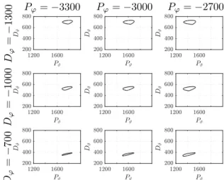
The domain of each control gain is divided into equal parts, and the maximal eigenvalue (λmax) of the mapping matrix at each gridpoint is calculated. Stability boundaries are given by the contourline whenλmax= 1. Fig. 3 represents the stable domains in the plane Pϑ, Dϑ for different pairs of (Pϕ, Dϕ). Stable domain are inside the contourlines.
3.2 Stabilizability
The wheel radius and the distance between the ground and the board have an important effect on the stability of the system. It is assumed, that a critical time delay exists for givenRandh: no control gains can stabilize the system for delays larger than the critical delay. This critical feedback delay was determined numerically for each combination of R and h, and the so-called stabilizability diagram was determined. Since stability is the function of the system parameters, e.g. mass, and dimensions of the balancing person, the stabilizability diagram has to be constructed for each subject separately.
Pϕ=−3300 Pϕ=−3000 Pϕ=−2700
Dϕ=−1300Dϕ=−1000Dϕ=−700
Fig. 3. Stability map for the parameters of S1 (Table 1, τ= 0.15 s,R= 0.25 m,h= 0.025 m).
3.3 Search algorithm
In order to determine the critical delay for a fixed pair (R, h), a numerical search algorithm was developed. The structure of the algorithm is shown in Fig. 4. As the first step, initial parameters have to be set, which are collected in Table 3. The discretization time step for the semidiscretization was ∆t = τ /r with delay resolution r= 10. This way the human nervous system is modelled as a digital controller with sampling frequency equal tor/τ. After pre-processing, all the four control gains are per- turbed by±0.1%. This gives 34 = 81 different cases. The maximal eigenvalue of the corresponding mapping matrix is calculated numerically for all the 81 cases, and the one with the smallest absolute value is selected as a new set point. In the next step, these new control parameters are perturbed again by ±0.1%, and the steps are repeated.
The process is terminated, when the chosen eigenvalue belongs to the original control gains (control gains of the previous step). This means that the global minimum is found associated with a given time delay. If this eigenvalue is lower than 1, time delay is increased with 0.01 s and the process is repeated. If the largest eigenvalue becomes greater than 1, then the process is stopped, and it is declared that there are no stabilizing control parameters for the given delay, i.e., this is the critical delay. The procedure is then performed for the next board distance h.
As shown by the experiments, balancing trials are more difficult, when the board-floor distance is large (i.e., h is small). Based on this observation, the algorithm starts with h=−0.05m for all R, and after finding the critical time delay for this combination, h is increased by one step and τ is decreased with 0.02 s lower than the previ- ously determined critical feedback delay, while the control parameters are held constant. These values are used as initial values for the next wheel radius-board distance configuration. When the radiusRis increased by one step, then the default initial values are used for the feedback delay and the control parameters.
ℎ<𝑅 𝜏=𝜏𝑐𝑟𝑖𝑡−0.02𝑠
Fig. 4. Search algorithm.
3.4 Evaluation of stabilizability diagrams
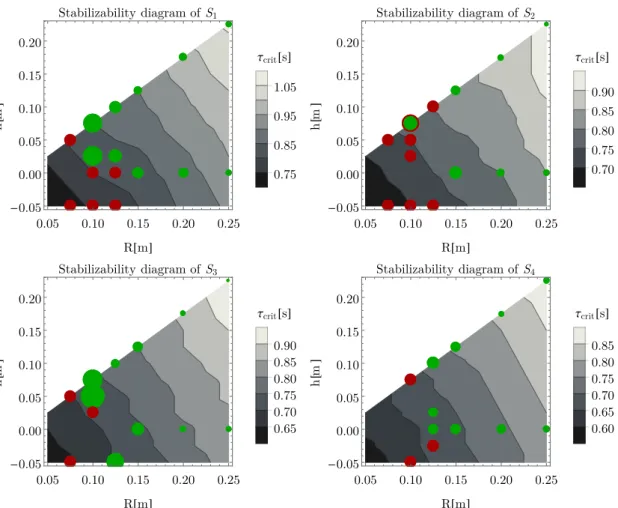
Stabilizability diagrams created using the parameters of S1, S2, S3 and S4 (Table 1) can be seen in Fig. 7.
Contourlines show, that the greater the wheel radius and the lower the board is positioned, the higher the critical time delay, therefore the easier the balancing task. The largest time delay belongs to the lowest position of the wheel having 250 mm radius, therefore this is the most stable configuration from balancing point of view. For instance, Fig. 7 shows that if the reaction time of S1 is lower than 1.05 s, then there exist control gains which can stabilize the equilibrium.
4. MEASUREMENT
In order to validate the model-based derivations, real balancing trials were performed in a systematic way.
OptiTrack camera system with 8 cameras was used to capture the motion four human subjects standing on the balance board. The sampling frequency was 120 Hz. Three reflective markers were fixed to the balance board and 5 markers were placed on the subject as shown in Fig. 5.
The flowchart of the measurement is shown in Fig. 6.
Subjects were asked to balance themselves for 60 seconds with open eyes. After 60 seconds, the trial was declared to be successful, and the next combination of (R, h) was set.
Balancing subjects have to balance with clasped hands behind their back, and try to keep their legs stretched.
Fig. 5. Position of markers used during the measurement (denoted by red arrows).
Reaction time test
Balance board – first configuration
R = 250 mm h = 0 mm
R = constant Minimum and maximum set of h
Both of them is successful One of them is
successful None of them is
successful
R is one size smaller Finding the stable point with halving
END START
Fig. 6. Steps of the measurement.
According to the mechanical model, the pin is located at the ankle, therefore the subjects were instructed to press their sole to the board in order to prevent the relative motion between the feet and the balance board.
According to Fig. 6, first the reaction time delay was measured using a reaction time measurement set. This device consists of a box with lights switching on and of randomly and can measure the time between a flash of the light signal and a response pedal push. Subjects were asked to push two pedals with their feet when the light is switched on. This way, the reaction time between a visual information and an actuation at the feet is measured. Each
0.05 0.10 0.15 0.20 0.25 -0.05
0.00 0.05 0.10 0.15 0.20
R[m]
h[m]
Stabilizability diagram ofS1
τcrit[s]
0.75 0.85 0.95 1.05
0.05 0.10 0.15 0.20 0.25 -0.05
0.00 0.05 0.10 0.15 0.20
R[m]
h[m]
Stabilizability diagram ofS2
τcrit[s]
0.70 0.75 0.80 0.85 0.90
0.05 0.10 0.15 0.20 0.25 -0.05
0.00 0.05 0.10 0.15 0.20
R[m]
h[m]
Stabilizability diagram ofS3
τcrit[s]
0.65 0.70 0.750.80 0.85 0.90
0.05 0.10 0.15 0.20 0.25 -0.05
0.00 0.05 0.10 0.15 0.20
R[m]
h[m]
Stabilizability diagram ofS4
τcrit[s]
0.60 0.65 0.700.75 0.80 0.85
Fig. 7. Stabilizability diagrams. Greyscale indicates the critical delay for the mechanica model, red and green circles indicates successfull and failed trials, respectively.
subject performed 10 reaction time measurements. The measured reaction times were in the range of 0.2 . . . 0.4 s.
In order to reduce the effect of learning, the subjects have the opportunity to practice balancing on the first config- uration (R = 250 mm, h= 0 mm) for 2 minutes before the measurement, as shown in Fig. 6. Then the balancing trials were started, the subject had to stand for 60 seconds on the first configuration. If the trial was successful, then the board distance was changed to the lowest position and another balancing trial was performed. If both of the balancing trials were successful, then the radiusRwas set by one size smaller, and the subject had to balance on the highest and lowest board distances, again. If only one of these trials were successful, then the stability bound- ary was found with halving method. The measurement is terminated, when balancing is not successful neither on the highest nor on the lowest board distances. The results are shown in Fig. 7. Different stabilometry parameters can be defined to describe and compare balancing skills (Nagym´at´e and Kiss, 2016; Nagym´at´e et al., 2018), here, we used the standard deviation of the angular oscillation.
Green circles indicate successful trials, the size of the circle is proportional to the standard deviation of the angular oscillationsϑof the balance board. Red circles indicate the pairs (R, h) where the balancing trial was not successful, i.e., the subjects could not balance themselves for 60 s. The
boundary between the green and red circles indicate the boundary of stabilizability. As can be seen, this bound- ary is parallel to the contour curves of the theoretically estimated critical delay.
Standard deviations at the lower settings of the board are smaller than at higher configurations, which agrees with the results obtained from the mechanical model. In case of wheels withR= 0.075 m, 0.1 m and 0.125 m, a raised edge was manufactured, therefore negativehvalues were tested, too. It can be seen, that balancing is more complicated when his negative. For the parameter combination R = 0.1 m and h = 0.075 m, subject 2 were able to balance on the board for 45 s. This trial is less unstable than the ones denoted by red color, but still cannot be considered stable. Therefore this parameter point is indicated by a green circle with red edge in the diagram associated with S2.
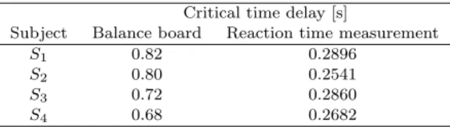
Comparison of the critical time delays obtained by the balance board measurements and the reaction times are shown in Table 4 for the different subjects. It can be seen that the balance board experiments indicate about three- times larger critical delays than the reaction time measure- ments. This discrepancy indicates that the reaction delay during balancing on a balance board might be of different nature than the delay measured during the reaction time measurements.
Table 4. Critial delays obtained via the stabi- lizability diagram of the balance board and by
direct reaction time measurements
Critical time delay [s]
Subject Balance board Reaction time measurement
S1 0.82 0.2896
S2 0.80 0.2541
S3 0.72 0.2860
S4 0.68 0.2682
5. CONCLUSIONS
Comparison of the critical delay obtained by the stabi- lizability analysis of the mechanical model of standing on a balance board in the frontal plane combined with balancing trials by four subjects and direct reaction time measurements for the same subjects was presented. The re- sults shown in Table 4 indicates that the critical delay de- termined using the mechanical model is about three times larger than the corresponding measured reaction times.
This discrepancy indicates that balancing on a balance board can be a more complex tasks than pushing a pedal by the feet during a reaction time test. Another explana- tion for the discrepancy might be that the model under analysis involves many simplifications. Namely, the model does not involves the sensory and actuation uncertainties during the balancing projects. These uncertainties would clearly decrease the corresponding critical delay. Further- more, a proportional-derivative control concept was as- sumed, which is a relatively simple control algorithm. The study of more sophisticated control concepts, such as the event-driven intermittent controller analyzed in Asai et al.
(2009) or the acceleration feedback from Insperger et al.
(2013), will be the object of further research.
ACKNOWLEDGMENT
This work was supported by the ´UNKP-17-2-I New Na- tional Excellence Program of the Ministry of Human Ca- pacities and by the Higher Education Excellence Program of the Ministry of Human Capacities in the frame of Biotechnology research area of Budapest University of Technology and Economics (BME FIKP-BIO).
REFERENCES
A. Silder, B. Whittington, B.H. and Thelen, D.G. (2007).
Identification of passive elastic joint moment-angle rela- tionships in the lower extremity.Journal of Biomechan- ics, 40, 2628–2635.
Asai, Y., Tasaka, Y., Nomura, K., Nomura, T., Casadio, M., and Morasso, P. (2009). A model of postural control in quiet standing: robust compensation of delay-induced instability using intermittent activation of feedback con- trol. PLOS ONE, 4, 1–14.
Bingham, J.T., Choi, J.T., , and Ting, L.H. (2011). Stabil- ity in a frontal plane model of balance requires coupled changes to postural configuration and neural feedback control. Journal of Neurophysiology, 106, 437–448.
Chagdes, J.R., Rietdyk, S., Haddad, J.M., Zelaznik, H.N., Cinelli, M.E., Denomme, L.T., Powers, K.C., and Ra- man, A. (2016). Limit cycle oscillations in standing
human posture. Journal of Biomechanics, 49, 1170–
1179.
de Leva, P. (1996). Adjustment to zatsiorsky-seluyanovs segment inertia parameters. Journal of Biomechanics, 29, 1221–1230.
Goodworth, A. and Peterka, R. (2010). Influence of stance width on frontal plane postural dynamics and coordination in human balance control. Journal of Neurophysiology, 104, 1103–1118.
Hajdu, D., Milton, J., and Insperger, T. (2016). Ex- tension of stability radius to neuromechanical systems with structured real perturbations. IEEE Transactions on Neural Systems and Rehabilitation Engineering, 24, 1235–1242.
Hwang, S., Agada, P., Kiemel, T., and Jeka, J.J. (2016).
Identification of the unstable human postural control system. Frontiers in Systems Neuroscience, 10, 22.
Insperger, T., Milton, J., and Stepan, G. (2013). Acceler- ation feedback improves balancing against reflex delay.
Journal of The Royal Society Interface, 10(79).
Insperger, T. and Stepan, G. (2011). Semi-Discretization for Time-Delay Systems - Stability and Engineering Applications. Springer, New York.
Loram, I. and Lakie, M. (2002). Direct measurement of human ankle stiffness during quiet standing: the intrinsic mechanical stiffness is insufficient for stability.
The Journal of Physiology, 545, 1041–1053.
Maurer, C. and Peterka, R.J. (2005). A new interpretation of spontaneous sway measures based on a simple model of human postural control. Journal of Neurophysiology, 93, 189–200.
Milton, J.G., Ohira, T., Cabrera, J.L., Fraiser, R.M., Gyorffy, J.B., Ruiz, F.K., Strauss, M.A., Balch, E.C., Marin, P.J., and Alexander, J.L. (2009). Balancing with vibration: A prelude for ”drift and act“ balance control.
PLoS One, 4, e7427.
Molnar, C.A., Zelei, A., and Insperger, T. (2017). Estima- tion of human reaction time delay during balancing on balance board. InProceedings of 13th IASTED Interna- tional Conference on Biomedical Engineering (BioMed), 195.
Nagym´at´e, G. and Kiss, R.M. (2016). Parameter reduc- tion in the frequency analysis of center of pressure in stabilometry. Periodica Polytechnica, 60(4), 238–246.
Nagym´at´e, G., Orlovits, Z., and Kiss, R. (2018). Reliability analysis of a sensitive and independent stabilometry parameter set. PLoS One, e0195995.
Riener, R. and Edrich, T. (1999). Identification of passive elastic joint moments in the lower extremities. Journal of Biomechanics, 32, 539–544.
Stepan, G. (2009). Delay effects in the human sensory system during balancing. Philosophical Transactions of the Royal Society A, 367, 1195–1212.
Suzuki, Y., Nomura, T., Casadio, M., and Morasso, P.
(2012). Intermittent control with ankle, hip, and mixed strategies during quiet standing: A theoretical proposal based on a double inverted pendulum model. Journal of Theoretical Biology, 310, 55–79.
Winter, D.A., Patla, A.E., Ishac, M., and Gielo-Perczak, K. (1998). Stiffness control of balance in quiet standing.
Journal of Neurophysiology, 80, 1211–1221.
Yoon, Y.S. and Mansour, J.M. (1982). The passive elastic moment at the hip. J. of Biomechanics, 15, 905–910.