This article is published with Open Access at www.akademiai.com DOI: 10.1556/168.2019.20.3.2
Introduction
The study of complex systems such as vegetation, fau- nas, landscapes, pedosphere, etc. with the aim to detect and understand the causes of their variation, from site to site or during time, is always based on the use of objects called operational geographic units (OGUs). The size and shape of the OGUs are often established according to the aim of the study (see Crovello 1981, Feoli and Zuccarello 1996 for references on OGUs), but often they are given by the nature of the OGUs, e.g., islands, watersheds, administrative units, industrial areas etc. The aim of this short note is to intro- duce the use of a family of similarity measures, called the Simpson’s similarity functions or nestedness-based similar- ity functions (NBSF), in order to cope with the fact that the differences between OGUs in terms of a set of features (spe- cies, plant communities, vegetation series, land use, land cover, etc.) could be due not only to replacement (cf. Podani and Schmera 2011, 2016) of the features from OGU to OGU, owing to the effects of specific environmental factors, but also to factors that would produce the so-called nestedness effect (Atmar and Patterson 1993, 1995, Ulrich et al. 2009, Ulrich and Almeida Neto 2012, Podani and Schmera 2011, 2016 and references therein), e.g., the loss of features in the same type of combination of features that would correspond to a typology (vegetation type, ecosystem type, urban type
etc.). These factors may be the extent of the area of OGUs, a small decrement or increment of soil fertility or moisture, an increment or decrement of human impact etc. and even inac- curate descriptions of OGUs. This short note is a follow-up of a previous paper whose aim was to find a classification of watersheds of the province of Almeria (Spain) on the ba- sis of vegetation series (Ibáñez et al. 2016). In that paper, we found that the classification based on Simpson’ s index provided a result more coherent with drainage and biocli- matic patterns than the classifications obtained by similarity functions (e.g., Jaccard, Sørensen) that do not account for nestedness (Nestedness Free Similarity Functions, NFSF).
We are aware of the potential importance of the nestedness concept in all branches of science, an example is given by Bustos et al. (2012) for the application in forecasting the industrial development, but we do not enter into discussing this aspect, nor the overall measures of nestedness in data matrices (Atmar and Patterson 1993, 1995), for which we refer to Ulrich et al. (2009) for a review, we just want to focus on the pairwise comparison between OGUs.
The Simpson’s similarity index
Simpson (1943) introduced an index to measure the re- semblance between faunas “to eliminate the effects of dis-
On the use of nestedness-based similarity functions (NBSF) to classify and/or order operational geographic units (OGUs)
E. Feoli
1,4, P. Ganis
1, J. J. Ibáñez
2and R. Pérez-Gómez
31Department of Life Sciences University of Trieste, 34127 Italy
2Research Centre on Desertification (Centro de Investigaciones sobre Desertificación, CIDE ,CSIC-UV), Km 405.
Apdo. Oficial 46113, Valencia, Spain
3Department of Topographic and Cartographic Engineering, Polytechnic University of Madrid (Departamento de Ingeniería Topográfica y Cartografía, Universidad Politécnica de Madrid, UPM), Camino de la Arboleda, s/n. Campus Sur UPM, Autovía de Valencia km. 7, E 28031 Madrid, Spain
4Corresponding author. Email: feoli@units.it
Keywords: Impoverishment; Inclusion; Maximum similarity; Nestedness; Set theory.
Abstract: In this paper, we want to support the idea of using a family of indices of similarity, that we call the Simpson’s family indices or nestedness-based similarity functions (NBSF) for comparing operational geographic units (OGUs) (phytosociologi- cal relevés, animal traps, watersheds, administrative units, industrial areas, islands etc.). In these cases, similarity-dissimilarity depends, in addition to factors that induce replacement, also on factors that produce reduction or increment in the number of features within the same typology of OGUs (e.g., extent, reduction of fertility, anthropogenic pressure etc.). To keep into consid- eration this aspect, the indices are defined to be equal to 1 when the OGUs are completely nested. The results of the application to four simulated data sets prove that, when the data set does not show clear nested pattern, the use of NBSF produces results similar to the nestedness-free similarity functions, however since NBSF clearly detect nested situations, we should prefer their use in the circumstances where we think important to put in evidence nestedness. In conclusion, we support the idea of using both types of indices in order to improve the knowledge about the structure of any data set.
Abbreviations: NBSF – Nestedness-Based Similarity Functions, NFSF – Nestedness-Free Similarity Functions, OGU – Operational Geographic Unit
crepancy in size between the faunas or samples“ (Simpson 1960). The index is given by the following formula:
(1a)
where j and k are two OGUs, a is the number of features shared by them and nj and nk are respectively their number of features. The index (1) is generally written in the follow- ing way:
(1b) where b and c, according the formalism of the two-way con- tingency table, are respectively the number of features pre- sent in j and lacking in k and the number of features present in k and lacking in j. The index is equal to 1 when the sets of features of two OGUs are equal, or when the set of one OGU includes completely the set of features of the other OGU, e.g., in case of complete nestedness, it is 0 when the two OGUs have no features in common.
In his papers, Simpson (1943, 1960) does not consider explicitly the concept of nestedness notwithstanding appar- ently the concept was introduced, according to Ulrich et al.
(2009) in biogeography, in the late 1930’s.
In case of complete nestedness, the similarity calculated with the traditional indices i.e., Jaccard, Sørensen, chord dis- tance etc., that we can call “nestedness free similarity func- tions” (NFSF), depends upon the differences between nj and nk (richness difference, cf. Podani and Schmera 2011, 2016), where nj is the number of features in the set j and nk is the number of features in set k. If we consider that complete nest- edness is realized when the absolute distance between two binary vectors is equal to the absolute difference between the totals of the vectors, e.g., nj and nk, it is easy to demonstrate that the Simpson’s index may also be written as:
(1c)
where D is the absolute distance between j, k, Djk min is the minimum possible distance between them (the richness dif- ference, see Podani and Schmera, 2011), and Dik max is nj+nk
(i.e., a = 0).
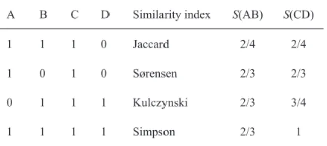
By the application of the “nestedness free similarity func- tions” (NFSF) it happens, as shown in Table 1, that two ob- jects (A and B) may have the same similarity-dissimilarity of other two objects (C and D), notwithstanding the pattern of features is completely different in the two pairwise com- parisons. In fact, A and B show replacement (2 min(b, c) = 2, cf. Podani and Schmera 2011) while C and D show complete nestedness (b or c = 0). If we use Jaccard’s index (Podani 2000) the similarity between the objects A-B, and C-D is the same: S(AB) = S(CD) = 2/4. If we apply the Kulczynski in- dex (Podani 2000) the two values are different S(AB) = 2/3, S(CD) = 3/4, however, the index does not inform about the fact that in the case of C and D there is complete nestedness.
If we apply the Simpson’s index, S(AB) = 2/3, S(CD) = 1, the
two similarity measures are different and in the second case (S(CD)) being equal to one, it informs that there is complete nestedness, i.e., there is no replacement.
The Simpson’s index is used by Baselga (2010) to calcu- late the “nestedness-resultant component” of Sørensen dis- similarity index, becoming a key tool and topic of what we can call the “beta diversity and nestedness dispute” (Baselga 2010, Ulrich and Almeida Neto 2012, Carvalho et al. 2013, Legendre 2014, Baselga and Leprieur 2015, Podani and Schmera 2016 and references therein). We do not want to enter such a dispute that looks well clarified by the papers of Legendre (2014) and Podani and Schmera (2016), but, as we have said in the Introduction, we want only to present the concept of “nestedness-based similarity function” (NBSF) as a generalization of the pairwise Simpson’s index. For the discussion on the decomposition of NFSF into replace- ment, nestedness, richness components, on the basis of the formalism of the two-way contingency table, we refer to the above mentioned papers (e.g., Baselga 2010, Legendre 2014, Baselga and Leprieur 2015, Podani and Schmera 2011, 2016).
The family of nestedness based similarity functions (NBSF)
The Simpson index can be interpreted as the ratio be- tween two scalar products, the first corresponding to the value calculated by the actual pattern of distribution of the feature among two objects, j and k, and the second corresponding to the value calculated considering the pattern of the features in case of complete nestedness. Formula 1) is actually the ratio between the scalar product a and the scalar product (min(nj, nk)) that is realized when two vectors of features describing j and k would be completely nested. Thus, being the index of Simpson a ratio between two scalar products and being the scalar product a basic index of similarity (see Orlóci 1978, Podani 2000) we can say that the index of Simpson belongs to a family of similarity indices that we can call the Simpson’s family indices and that could be written in the following way:
(2) where Sjk is the observed similarity between the objects j and k and Sjk max is the maximum similarity they would have when j and k are completely alike or when the features nj and
A B C D Similarity index S(AB) S(CD)
1 1 1 0 Jaccard 2/4 2/4
1 0 1 0 Sørensen 2/3 2/3
0 1 1 1 Kulczynski 2/3 3/4
1 1 1 1 Simpson 2/3 1
Table 1. Two pairs of OGUs A versus B and C versus D, showing respectively replacement and nestedness.
nk are arranged in a nested way (the set of features nj is com- pletely included in the set of features nk or vice versa, i.e., in terms of two-way contingency table b or c is equal to zero).
In this last case there is no replacement of features but only impoverishment or enrichment.
Any “nestedness free” similarity index (NFSF) ranging between 0 and 1 (0 = no similarity, 1= maximum similar- ity) can be used in formula 2). Of course, we cannot use the Simpson’s index, that actually is a measure of nestedness, because in this case it may easily happen that the ratio in formula 2) could be higher than 1 (e.g., when a/min(nj,nk) >
(nj/nk or nk/nj).
It is easy to show that among the NFSFs, if we use the one of Sørensen (Podani 2000), formula 2) becomes the in- dex of Simpson. Formula 2) can be written also as formula 1c) when a dissimilarity function is chosen instead similarity (see Appendix).
In terms of fuzzy set theory (Zadeh 1965), formula 2) may also be called the degree of nestedness or “nestedness degree”. Its complement to one:
Rjk(n) = 1 – Sjk(n) (3) can be considered a measure of non-nestedness, i.e., replace- ment (Rjk(n)), the “non-nestedness component”, or in other words, the relative gap between the actual similarity and the maximum similarity two OGUs may have in case of being alike or being nested. Baselga (2010) for the Sørensen index in formula 2) and 3) suggests that the difference:
Djk(n) = Sjk(n) – Sjk (4) should be called the “nestedness resultant dissimilarity”, it is 0 when j = k and when nj = nk, irrespective the value of a (the common features between two OGUs) since in this case Sjk max will be equal to 1. It is to be emphasized that Baselga (2010) is suggesting Djk(n) as difference between the comple- ment of the Sørensen’s index (i.e., the Sørensen dissimilar- ity index) and the complement of the index of Simpson (the Simpson dissimilarity index). However owing to the draw- back mentioned above, i.e., that it could be 0 irrespective the value of a, Djk(n) is useless if used alone, but it could be use- ful if used in ternary plots (e.g., Podani and Schmera 2011) that can be obtained thanks to the following relationship very easy to demonstrate:
Rjk(n) + Djk(n) + Sjk = 1 (5) In case of nj=nk, in the ternary plot a pair of OGUs will be toward Rjk(n) if b,c > a, and will be toward Sjk when b,c < a.
According to formula 4), formula 2) can also be written as:
Sjk(n) = Sjk + Djk(n) (6) that is to say, any NBSF is given by its “nestedness free simi- larity function” plus the corresponding “nestedness resultant dissimilarity” or better, in terms of similarity, the loss of simi- larity due to the loss or increment of features (i.e., due to the richness difference). Since Sjk(n) can be equal to Sjk only if nj = nk, i.e., when Sjkmax is equal to 1, we can conclude that given a certain a (i.e., the number of features in common be- tween j and k), Djk(n) depends on the richness difference, or
in other terms, given a certain a, Djk(n) is increases if |nj – nk| increases. However at parity of a, the nestedness measured by formula 2) (Sjk(n)) depends on the formula of NFSF used, if we use the formula of Sørensen, formula 2) reduces to the Simpson formula (1)) and it remains constant if the min(nj, nk) remains constant even if the richness difference is increas- ing, while in the case of the Jaccard’s function it is easy to show that Sjk(n) is increasing as the richness difference in- creases even if the min(nj, nk) remains constant. The choice of one NFSF is a matter of the weight we want to give to rich- ness differences. It is easy to verify what it is happening with the application of different NFSF by the use of simple simu- lated data or by simple algebra just remembering that, when calculating the Sjkmax, a (the number of features in common) is always equal to min(nj, nk).
Comparison between the application of NBSF and NFSF
Data
To compare the performance of the NBSF with respect to the NFSF we use four simulated data sets. They contain 15 vectors that represent OGUs described by features arranged in 4 different ways:
1) the first simulated data set presents a classical situation of replacement along an hypothetical gradient with only the last vector nested in the previous one (Table 2);
2) the second simulated data set shows two complete nested situations in which the two OGUs with the maximum number of features are more different from each other than from OGUs in their own group, i.e., the group they include (Table 3);
3) the third simulated data set presents two complete nested situations in which the two OGUs richest in features are more similar to each other than to those nested with them (Table 4);
4) the fourth simulated data set presents two situations with a very high nested component, but not with complete nested- ness (Table 5). This last data set simulates the study on the land system of Almeria (Spain) by Ibanez et al. (2016) and Feoli et al. (2017) based on watersheds as OGUs, whose re- sults inspired this paper.
Data analysis
The 15 vectors (hypothetical OGUs) of simulated data have been compared by formula 2) in which Sjk and Sjkmax have been calculated by the Sørensen index, Jaccard index and angular separation (cosine) (Podani 2000) and by the same indices in their original form (NFSF). To the similar- ity matrices we have applied the group average and complete linkage clustering algorithms (Podani 2000).
Results
Figures 1, 2, 3 and 4 show the results of the application of formula (2) and of the respective “nestedness free similarity functions” (NFSF) to the data of Tables 2, 3, 4 and 5. Each
figure presents only two dendrograms, obtained by average linkage cluster analysis by the Sørensen index implemented in formula (2) and applied as a NFSF, respectively. We have chosen to present only these two dendrograms for two rea- sons: a) the use of Sørensen index gives exactly the Simpson’s index; b) the dendrograms based on all the three resemblance functions, namely Sørensen, Jaccard and “cosine”, are all top- ologically very similar for each data set, when applied with formula (2) and when applied directly, irrespective the two different methods of clustering, i.e., the average and complete linkage clustering methods (Podani 2000).
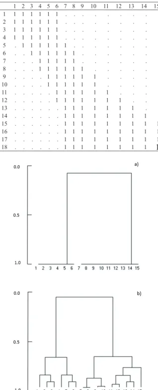
It is clear from Fig. 1, corresponding to Table 2, where the simulated data represent a typical gradient with replacement, that the results of the application of formula (2) and of the corresponding NFSF are almost the same.
Figure 2 shows that formula (2), applied to Table 3, where the simulated binary data represents two complete nested situations in which the two richest vectors (columns 6 and 7) have a lower similarity with each other than with the cor- responding nested vectors, gives two well separated clusters with the OGUs at same level of similarity. Each cluster con- tains all the OGUs belonging to a nested situation. In this case the dendrograms of all the NFSF show the same two main clusters obtained by formula (2), the differences being that these dendrograms show the pattern of similarity within each cluster: a pattern that formula (2) is not able to show.
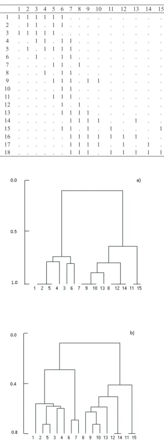
Figure 3 shows that formula (2), applied to Table 4, a case of two complete nested situation, gives different results with respect those obtained by the NFSF. As a matter of fact, while by NFSF the two OGUs richest in the number of features (6, 7 with 13 and 15 features, respectively) are belonging to the same cluster, by formula (2) each of them belongs to the clus- ter corresponding to the nested situation of which they are the elements with the highest richness.
Figure 4 shows the results of cluster analysis correspond- ing to Table 5, a case where the nestedness is incomplete within two main clusters. The results are similar to those of Figure 3, however, the dendrogram a) is able to detect and to show the cases of complete nestedness.
Discussion and conclusions
Despite the many indices proposed in the literature to measure nestedness (see Ulrich et al. 2009, Urlich and Almeida-Neto 2012, Podani and Schmera 2011, 2012, 2016 for reviews), there is no mention of NBSF as applied for clas- sification purposes outside biogeography, although they may have relevance when we want to classify OGUs that are sub- jected to nestedness effects.
The results obtained by simulated data support the idea that NBSF would give the same results of NFSF if there is not complete nestedness in the data sets or in their subsets, with the advantage of showing very clearly the cases of complete nestedness. However, in the case of complete nestedness between the OGUs of the same group (cluster), the dendro- grams obtained by NBSF are not able to show the pattern of similarity between the OGUs. For this reason, we suggest to
Table 2. A simulated binary data considering a regular replace- ment and one nested situation (vector 14 includes vector 15).
1 2 3 4 5 6 7 8 9 10 11 12 13 14 15
1 1 . . . .
2 1 1 . . . .
3 . 1 1 . . . .
4 . . 1 . . . .
5 . . 1 1 . . . .
6 . . . 1 . . . .
7 . . . 1 1 . . . .
8 . . . 1 1 . . . .
9 . . . . 1 1 . . . .
10 . . . . 1 1 . . . .
11 . . . 1 1 . . . .
12 . . . 1 1 . . . .
13 . . . 1 1 1 . . . .
14 . . . 1 1 . . . .
15 . . . 1 1 1 . . . . .
16 . . . 1 1 1 . . . . .
17 . . . 1 1 1 . . . .
18 . . . 1 1 1 . . . .
19 . . . 1 1 . . . .
20 . . . 1 1 . . .
21 . . . 1 1 . . .
22 . . . 1 1 1 . .
23 . . . 1 1 . .
24 . . . 1 1 1 .
25 . . . 1 1 .
26 . . . 1 1
Figure 1. Dendrogram of NBSF (a) and of NFSF (b) for data in Table 2. The Sørensen index and clustering by average linkage within merged groups have been used.
Figure 1. Dendrogram of NBSF (a) and of NFSF (b) for data in Table 2. The Sørensen index and clustering by average linkage have been used.
use always the NBSF and the corresponding NFSF to have both: the evidence of nested situations, when they are present in the data set, and the nested free similarity pattern of the set of OGUs. In the paper of Ibanez et al. (2016), we have found that the use of a NBSF has shown a classification of OGUs
more coherent with the drainage pattern of the watersheds system of the area and with climatic data.
We conclude by saying that the concept of nestedness is a fuzzy concept, in the sense that the nestedness of any two vectors measured by NBSF, in which n objects are described Table 3. Simulated binary data for a nested situation in which the
two richest vectors (6 and 7) have a lower similarity with each other than with the corresponding nested vectors..
1 2 3 4 5 6 7 8 9 10 11 12 13 14 15
1 1 1 1 1 1 1 . . . .
2 1 1 1 1 1 1 . . . .
3 1 1 1 1 1 1 . . . .
4 1 1 1 1 1 1 . . . .
5 . 1 1 1 1 1 1 . . . .
6 . . 1 1 1 1 1 1 . . . .
7 . . . 1 1 1 1 1 . . . .
8 . . . 1 1 1 1 1 1 . . . .
9 . . . . 1 1 1 1 1 1 . . . . .
10 . . . . 1 1 1 1 1 1 . . . . .
11 . . . 1 1 1 1 1 1 . . . .
12 . . . 1 1 1 1 1 1 1 . . .
13 . . . 1 1 1 1 1 1 1 . .
14 . . . 1 1 1 1 1 1 1 1 .
15 . . . 1 1 1 1 1 1 1 1 1
16 . . . 1 1 1 1 1 1 1 1 1
17 . . . 1 1 1 1 1 1 1 1 1
18 . . . 1 1 1 1 1 1 1 1
1
Figure 2. Dendrogram of NBSF (a) and of NFSF (b) for data in Table 3. The Sørensen index and clustering by average linkage within merged groups have been used.
Figure 2. Dendrogram of NBSF (a) and of NFSF (b) for data in Table 3. The Sørensen index and clustering by average linkage have been used.
Table 4. Simulated binary data for a nested situation in which the two richest vectors (6 and 7) have a higher similarity with each other than with the corresponding nested vectors.
1 2 3 4 5 6 7 8 9 10 11 12 13 14 15
1 1 1 1 1 1 1 . . . .
2 1 1 1 1 1 1 . . . .
3 . 1 1 1 1 1 . . . .
4 . . 1 1 1 1 1 . . . .
5 . . . 1 1 1 1 . . . .
6 . . . . 1 1 1 . . . .
7 . . . . 1 1 1 . . . .
8 . . . 1 1 . . . .
9 . . . 1 1 . . . .
10 . . . 1 1 . . . .
11 . . . 1 1 . . . .
12 . . . 1 1 1 . . . .
13 . . . 1 1 1 1 . . . .
14 . . . 1 1 1 1 . . . . .
15 . . . 1 1 1 1 1 . . . .
16 . . . 1 1 1 1 1 1 1 . .
17 . . . 1 1 1 1 1 1 1 1 .
18 . . . 1 1 1 1 1 1 1 1 1
Figure 3. Dendrogram of NBSF (a) and of NFSF (b) for data in Table 4. The Sørensen index and clustering by average linkage within merged groups have been used.
Figure 3. Dendrogram of NBSF (a) and of NFSF (b) for data in Table 4. The Sørensen index and clustering by average linkage have been used.
by m binary characters, is actually expressing a degree of be- longing of the matrix of the two vectors to the set of matrices of complete (perfect) nestedness. The use of ternary plots of Podani and Schmera (2016) by considering several possibili- ties: 1) only the single pairs of OGUs, 2) clusters of OGUs, 3) all the pairs of OGUs or 4) the averages values of pairs in clusters or 5) the averages of all the pairs in the matrices D, R and S (following formula 5)), may show the relationships between nestedness, replacement and similarity to fully high- light the similarity pattern within sets of OGUs.
Aknowledgment: We thank J. Podani for reading and com- menting the manuscript.
References
Atmar, W. and B.D. Patterson. 1993. The measure of order and disorder in the distribution of species in fragmented habitat.
Oecologia 96:373–382.
Atmar, W. and B.D. Patterson. 1995. The nestedness temperature cal- culator: a visual basic program, including 294 presence-absence matrices. AICS Research Inc, University Park, New Mexico, USA and the Field Museum, Chicago, IL, USA.
Baselga, A. 2010. Partitioning the turnover and nestedness compo- nents of beta diversity. Glob. Ecol. Biogeogr. 19:134–143.
Baselga, A. and F. Leprieur. 2015. Comparing methods to separate components of beta diversity. Meth. Ecol. Evol. 6(9):1069–1079.
Bustos, S., C. Gomez, R. Hausmann and C.A. Hidalgo. 2012. The dynamics of nestedness predicts the evolution of industrial eco- systems. PLoS One 7(11): e49393.
Carvalho, J.C., P. Cardoso, P.A.V. Borges, D. Schmera and J. Podani.
2013. Measuring fractions of beta diversity and their relation- ships to nestedness: a theoretical and empirical comparison of novel approaches. Oikos 122(6):825–834.
Crovello, T.J. 1981. Quantitative biogeography: an overview. Taxon 30:563–575.
Feoli, E. and V. Zuccarello. 1996. Spatial pattern of ecological pro- cesses: the role of similarity in GIS applications for landscape analysis. In: M. Fisher, H. Scholten and D. Unwin (eds), Spatial Analytical Perspectives on GIS. Taylor and Francis, London. pp.
175–185.
Feoli, E., R. Pérez-Gómez, C. Oyonarte and J.J. Ibáñez. 2017. Using spatial data mining to analyze area-diversity patterns among soil, vegetation, and climate: A case study from Almería, Spain.
Geoderma 287:164–169.
Ibáñez, J.J., R. Pérez-Gómez, P. Ganis and E. Feoli. 2016. The use of vegetation series to assess α and β vegetation diversity and their relationships with geodiversity in the province of Almeria (Spain) with watersheds as operational geographic units. Plant Biosystems 150(6):1395–1407.
Legendre, P. 2014. Interpreting the replacement and richness dif- ference components of beta diversity. Glob. Ecol. Biogeogr.
23:1324–1334.
Podani, J. 2000. Introduction to the Exploration of Multivariate Biological Data. Backhuys, Leiden, NL.
Podani, J. and D. Schmera. 2011. A new conceptual and methodolog- ical framework for exploring and explaining pattern in presence- absence data. Oikos 120:1625–1638.
Podani, J. and D. Schmera. 2012. A comparative evaluation of pair- wise nestedness measures. Ecography 35:889–900.
Table 5. Simulated binary data for a nested situation in which the two richest vectors (6 and 7) have a higher similarity with each other than with the corresponding nested vectors, there is a very high nested component, but not a complete nestedness as in Table 4.
1 2 3 4 5 6 7 8 9 10 11 12 13 14 15
1 1 1 1 1 1 1 . . . .
2 . 1 1 . 1 1 . . . .
3 1 1 1 1 1 . . . .
4 . . 1 1 . 1 1 . . . .
5 . 1 . 1 1 1 1 . . . .
6 . . 1 . . 1 1 . . . .
7 . . . . 1 1 . 1 . . . .
8 . . . 1 . 1 1 . . . .
9 . . . . 1 1 1 . 1 1 . . . . .
10 . . . 1 1 . . . .
11 . . . . 1 1 1 . . . .
12 . . . 1 . 1 . . . .
13 . . . 1 1 1 1 . . . .
14 . . . 1 1 1 1 . . 1 . .
15 . . . 1 1 . 1 . 1 . . . 1
16 . . . 1 1 1 1 1 1 1 . .
17 . . . 1 1 1 1 . 1 . 1 .
18Figure 4. Dendrogram of NBSF (a) and of NFSF (b) for data in Table 5. The Sørensen index and . . . 1 1 1 . 1 1 1 1 1 clustering by average linkage within merged groups have been used.
Figure 4. Dendrogram of NBSF (a) and of NFSF (b) for data in Table 5. The Sørensen index and clustering by average linkage within merged groups have been used.
Nestedness-based similarity functions 229 Podani, J. and D. Schmera. 2016. Once again on the components of
pairwise beta diversity. Ecol. Informatics 32:63–68.
Orlóci, L. 1978. Multivariate Analysis in Vegetation Research. 2nd edition. Junk, The Hague.
Simpson, G.G. 1943. Mammals and the nature of continents. Amer.
J. Sci. 241:1–31.
Simpson, G.G. 1960. Notes on the measurement of faunal resem- blance. Amer. J. Sci. 258(2):300–311.
Ulrich, W and M. Almeida-Neto. 2012. On the meanings of nested- ness: back to the basics. Ecography 35:1–7.
Ulrich, W., M. Almeida-Neto and N. Gotelli. 2009. A consumer’s guide to nestedness analysis. Oikos 118:3–17.
Zadeh, L.A. 1965. Fuzzy sets. Inform. Control 8:338–353.
Received July 17, 2019 Revised September 13, 2019 Accepted October 7, 2019 Appendix
We show that formula (2) becomes the index of Simpson when the nestedness free similarity function is the index of Sørensen.
The index of Sørensen can be written according to the formalism of the 2 × 2 contingency table as:
Since the maximum similarity is given when there is complete nestedness (or complete similarity) for the index of Sørensen it is:
it follows that, according to formula (2), Sjk(n) for the index of Sørensen becomes:
that is the Simpson’s index as in formula (1).
Open Access statement. This is an open-access arti- cle distributed under the terms of the Creative Commons Attribution-NonCommercial 4.0 International License (https://creativecommons.org/licenses/by-nc/4.0/), which permits unrestricted use, distribution, and reproduction in any medium for non-commercial purposes, provided the original author and source are credited, a link to the CC License is provided, and changes – if any – are indicated.
Appendix
We show that formula 2) becomes the index of Simpson when the nestedness free similarity function is the index of Sørensen.
The index of Sørensen can be written according to the formalism of the 2 x 2 contingency table as:
𝑆�� = 2𝑎 2𝑎+𝑏+𝑐
Since the maximal similarity is given when there is complete nestedness (or complete similarity) for the index of Sørensen it is:
𝑆��𝑚𝑎𝑥=2(min�𝑛�,𝑛��)
2𝑎+𝑏+𝑐 = 2(a + min (b, c)) 2𝑎+𝑏+𝑐
it follows that, according to formula 2), S
jk() for the index of Sørensen becomes:
𝑆��(𝑣)=
2𝑎+2𝑎𝑏+𝑐 2(𝑎+ min(𝑏,𝑐))
2𝑎+𝑏+𝑐
= 𝑎 𝑎+ min (𝑏,𝑐) that is the Simpson’s index as in formula 1).
Appendix
We show that formula 2) becomes the index of Simpson when the nestedness free similarity function is the index of Sørensen.
The index of Sørensen can be written according to the formalism of the 2 x 2 contingency table as:
𝑆�� = 2𝑎 2𝑎 + 𝑏 + 𝑐
Since the maximal similarity is given when there is complete nestedness (or complete similarity) for the index of Sørensen it is:
𝑆��𝑚𝑎𝑥 =2(min�𝑛�, 𝑛��)
2𝑎 + 𝑏 + 𝑐 = 2(a + min (b, c)) 2𝑎 + 𝑏 + 𝑐
it follows that, according to formula 2), S
jk() for the index of Sørensen becomes:
𝑆��(𝑣)=
2𝑎 + 𝑏 + 𝑐2𝑎 2(𝑎 + min(𝑏, 𝑐))
2𝑎 + 𝑏 + 𝑐
= 𝑎 𝑎 + min (𝑏, 𝑐) that is the Simpson’s index as in formula 1).
We show that formula 2) becomes the index of Simpson when the nestedness free similarity function is the index of Sørensen.
The index of Sørensen can be written according to the formalism of the 2 x 2 contingency table as:
𝑆�� = 2𝑎 2𝑎+𝑏+𝑐
Since the maximal similarity is given when there is complete nestedness (or complete similarity) for the index of Sørensen it is:
𝑆��𝑚𝑎𝑥=2(min�𝑛�,𝑛��)
2𝑎+𝑏+𝑐 = 2(a + min (b, c)) 2𝑎+𝑏+𝑐
it follows that, according to formula 2), S
jk() for the index of Sørensen becomes:
𝑆��(𝑣)=
2𝑎+2𝑎𝑏+𝑐 2(𝑎+ min(𝑏,𝑐))
2𝑎+𝑏+𝑐
= 𝑎 𝑎+ min (𝑏,𝑐) that is the Simpson’s index as in formula 1).