EXAMPLE FOR 2D PLANE STRESS
Author: Dr. István Oldal
7. EXAMPLE FOR 2D PLANE STRESS
7.1. Analysis of a strap plate
Let us determine the stresses in the strap plate of the frame (see Figure 7.1). The plate is bolted to one beam by two bolts and to another beam by one bolt. Stresses, due to the con- tact relationship are neglected.
Figure 7.1: Frame
The frame is loaded by a force withF =200N magnitude. The frame is fixed together by the strap plates at both sides, thus one individual strap plate is loaded only with one-fourth of the force (see Figure 7.2). The thickness of the plate is:v=1,5mm.
The loads and the deformations are in the plane of the plate (in the range of the linear, elas- tic material model), thus we can apply the Plane Strain model.
Figure 7.2: Dimensions and load of the strap plate
7.2. Solution by ANSYS Workbench 12.1
In order to solve this specific problem – after starting the program – we have to choose the type of the problem in the project menu. In our case, we wish to carry out a strength check in static condition. Thus we choose the Static structural line (see in Figure 7.3). The selec- tion can be carried out either by double-clicking or dragging the chosen mode into the white field by holding on the left-click button. After the selection, the requested analysis mode appears in the Project Schematic (see in Figure 7.3.b).
As the window appears, we can specify a name for the task. The window includes six op- tions. By opening the Engineering Data the material constants can be set or modified. This program does not demand to set the material constants, but we have to aware that in this case, it operates with the default settings which are linear, elastic structural steel. By dou- ble-clicking on Geometry, the program starts the geometry module where we are able to draw, modify or import the investigated structure. By double-clicking on Model, we open
a) b) Figure 7.3: Project window
7.2.1. Geometry modeling
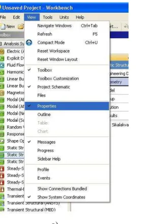
A planar deformation problem begins with the 2D modeling. This can be set before or after drawing the geometry in the Project Schematic. By clicking on Geometry, we can see the Property window on the left side of the screen and in its 16th line we can define the default 3D option to 2D (see in Figure 7.4.b). If the Properties of Schematic window is not visible, then if we click on View/Properties menu (see in Figure 7.4.a) it becomes visible.
After setting the dimension of the problem, we start the Design Modeler menu by double- clicking on Geometry in the Static Structural window. First of all, we have to define the unit (see in Figure 7.5).
The Design Modeler – similar to other 3D modeler software – builds up the models from layers and sketches by modifying them. Before drawing a sketch, we have to choose a
a) b) Figure 7.4: Setting the dimension of the problem
Figure 7.5: Selecting unit
plane to work with. The default plane, if we do not choose anything else, is the xy plane.
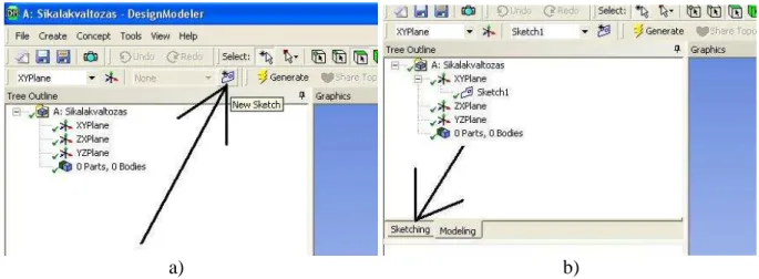
2D problems are compulsory drawn in this plane, since the program cannot define other planes in case of two-dimensional modeling. To draw a sketch, we have to click on New sketch icon (see in Figure 7.6.a), then in the left window – as a branch of the defined plane – Sketch1 appears. Let us now click on Sketching tab (see in Figure 7.6.b).
In order to have a better view over the sketch, we change our point of view from the de- fault axonometric view to a view which is perpendicular to the sketch by clicking on the icon shown in Figure 7.7.
Let us select Rectangle command in Draw window (Figure 7.8.a), and draw a rectangle, then with the Dimensions/General command (Figure 7.8.b) we appoint lines which are perpendicular to each other and we set the lengths of them to 40 and 10 mm in Details View window (Figure 7.9.a). We repeat these steps and we draw another rectangle (30x10mm) to the left corner of this rectangle (Figure 7.9.b).
We merge the two rectangles into one contour. Let us cut off the scrap line with the Mod- ify/Trim command shown in Figure 7.9.b. This line is the part of both rectangles (they cover each other) but it does not appear on the common contour, thus it has to be trimmed two times.
a) b) Figure 7.6: Creating new sketch
Figure 7.7: Setting the View perpendicular to the sketch
The rounding is carried out by the Modify/Fillet command. We start the rounding with cor- ners with 1mm radius. By selecting the command, we have to set the rounding radius (Fig- ure 7.10.a) and then we click on both lines of the corner in the sketch window. In our case, another option is if we draw the half circles with rounding command, but we have to be aware to set the radius to 4.99 mm, since the program cannot deal with connecting lines.
(These circles can be drawn in more steps and by the Modify/Trim command the edges and scrap lines can be cut off, but this method is quicker). After finishing the outer contour, we draw three circles with the Draw/Circle command. Then we set the diameters with the Di- mensions/Radius command and finally we relocate them with the Dimensions/Horizontal and Dimensions/Vertical commands. (The dimensions have to be designed with respect to the rule that negative or zero dimensions cannot be defined!)
a) b) Figure 7.8: Sketch menu
a) b) Figure 7.9: Dimensioning in details – Window and sketch
Now we have to make surfaces on the complete sketch (Figure 7.10.b). By clicking on Modeling tap (Figure 7.11.a) we exit the sketch drawing and then we execute Con- cept/Surfaces from sketches command by clicking on it (Figure 7.11.b).
After executing the command, the Details of SurfaceSk1 window appears on the left side of the screen (Figure 7.12).
a) b) Figure 7.10: Rounding command and the complete sketch
a) b) Figure 7.11: Exiting Sketch and making surfaces
We can see the name of the surface – which we are about to make – in the window (the program automatically creates a name). In the second line, we can choose the sketch that we use for making the surface. The selection can be carried out by either clicking on the chosen line of the sketch or clicking on the appropriate branch of the tree structure. In our case there is only one sketch, thus it is automatically selected, but in all the other three cases we have to accept our decision by clicking on Apply in Base Objects menu (Figure 7.12.a). The other options stay as default, we execute the Generate command (Figure 7.12.b) and our surface is already generated and appeared in the last branch of the tree structure as Surface Body (Figure 6.13.a). Then, we return to the project menu.
7.2.2. Finite Element Simulation
In the project module, by double-clicking on Model (Figure 7.14.) in the Static Structural window, the finite element module (Mechanical) starts. Make sure that you set the module to 2D modeling in the Properties of Schematic window of the Geometry menu (Figure 7.14.b).
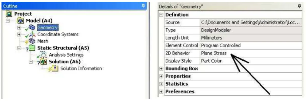
After starting the module, we have to define the type of the 2D problem. By clicking on the Geometry branch of the tree structure, the Details of Geometry window opens, where the options for 3D modeling becomes visible in the 2D Behavior settings (Figure 7.15). Let us select the default – Plane Strain – model.
a) b) Figure 7.12: Settings on Surface
a) b) Figure 7.13: The generated surface in the tree structure
Figure 7.14: Starting the finite element simulation
In Plane Strain model, we only have to define the thickness of the plate between each sur- face as parameters. By opening Geometry branch the existing bodies become visible, in our case the Surface Body. Let us click on it, and now we can see the details in the Details of Surface Body window. We have to set the thickness of the plate in the Thickness option (Figure 7.16). If we do not specify thickness, then the program automatically sets it to 1 mm (or does not execute the simulation and marks it with a question mark depend- ing on the version of the program)!
7.2.3. Meshing
As a first step of modeling, we have to discretize the model by creating a mesh. If we do not set the meshing parameters, the program will create a mesh with the default settings.
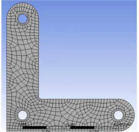
This method results rarely optimal mesh. In Figure 7.17, the mesh with default settings is shown.
Figure 7.15: Selecting 2D modeling
Figure 7.16: Setting the thickness
As we can see, the program built up the mesh using mostly rectangular elements with eight nodes. This element type – alongside with the size – are acceptable compared to the ge- ometry. However, in the corner with 1 mm radius – where the maximum stress is expected – smaller elements have to be specified.
If we wish to know the precise dimensions of the mesh, then we have to set it for our- selves. By right-clicking on the Mesh branch, the parameters of the mesh can be set under the upcoming Insert window. Firstly, we choose the element type with the Method com- mand (Figure 7.18.a).
In order to execute the command we have to select the body (if it is not the surface of a body but a surface model of a body the Workbench will model it as a body ‘Surface Body’) and then click on Method command (Figure 7.18.a). Then the Details window appears be- low, on the left corner, and we can carry out the settings.
Figure 7.17: Mesh with default settings
a)
b) c) Figure 7.18: Settings of the mesh
Unlike other finite element programs, not the element type has to be selected, but by defin- ing the parameters of the mesh, the program will automatically select element type fitting to the mesh. In the Method option (Figure 7.18.b) triangular and rectangular elements can be selected. In our case the rectangular elements are the most adequate. The order of the approximate functions (the numbers of the element nodes) can be set in the Element Mid- side Nodes option (Figure 7.18.c). In this specific case the quadratic approximation is needed since the planar model cannot be meshed with linear functions (it is not enclosed by linear lines). Let us select the rectangular element with eight nodes – including the nodes in the middle plane – and click on Kept.
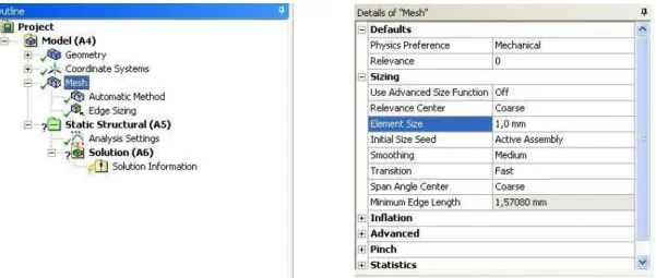
We have to define the element size if we do not wish to use the default element size. To define the average element size, we have to click on Mesh branch and in Details of Mesh window we can select Sizing/Element Size window and type in the value (Figure 7.19).
Taking into account the dimensions of the strap plate the average element size is set to 1 mm. This size is automatically reduced in the rounded corners, which is appropriate for the bores since we neglect the stresses related to the contact relationship (we would not obtain realistic results even if we enhanced the precision). By this setting (1mm) the element size will be reduced in the corners and we obtain more realistic results at the extremes.
Figure 7.19: Setting average element size
If we want to define different element size at the edges, surfaces, then we have to apply the Insert/Sizing command (Figure 7.20.a). After selecting the command, we have to choose the applicable geometry where we wish to set the size. In our case, this is the inner curve of the quarter circle and the curves of the two radiuses. The selecting has to be switched at the top icon menu (Figure 7.20.b). In the Details of Sizing window the selected curves have to be accepted by the Apply command and the element size – 0.2 mm – has to be typed into the Element Size option.
As it was mentioned earlier, we can execute the Generate Mesh (Figure 7.21.a) command and create our mesh (Figure 7.21.b).
7.2.4. Setting the boundary conditions a)
b) c) Figure 7.20: Setting the element size
a) b) Figure 7.21: Mesh generation and the complete mesh
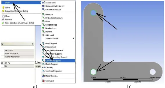
We can find the boundary conditions by right-clicking on the Static Structural branch and selecting Insert option. First of all, we define the constraints. The moment generated by a wood screw is neglected due to its irrelevance compared to the moment taken by the two bores. Thus the edges of the two unloaded bores are constrained in radial direction. We execute the Static Structural/ Insert/Cylindrical Support command (Figure 7.22.a).
After executing the commands, we select the two edges by the help of the icon in Figure 7.20.b. Normally, only one edge can be selected in the same time, but if we press on CTRL button, then more edges are possible to select. After the selection, we accept it by the Ap- ply command in the Details of Cylindrical Support window (Figure 7.23) we constrain the radial displacement (Fixed) and we allow the tangential displacement (Free).
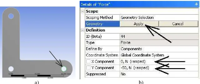
We define a force on the edge of the third bore. In the Workbench, we do not have to con- vert the force into distributed force system since if the force is applied on a line or edge the program automatically does that. After executing the Static Structural/ Insert/Force com- mand, we have to select the curve of the circle (Figure 7.24.a), and accept it with the Apply command (Figure 7.24.b). At the Define By option we can define the force vector by its components if we set it from Vector to Components. Let us change the y value to the mag-
a) b) Figure 7.22: Setting the constraints
Figure 7.23: Setting the constraints
7.2.5. Results
After setting the boundary conditions the simulation can be executed by the Solve com- mand. The requested results can be displayed after the simulation manually, but if we se- lect which results are we interested about, then these results will automatically displayed after the computation.
In this specific case, we would like to compute the equivalent stresses. If we know the equivalent stresses we can compare them to the given yield stress and decide whether the strap plate is suitable for such a load or not. In order to display these results we right-click on the Solution branch and we select the Insert/Stress/Equivalent option (Figure 7.25).
The computation of the problem can be initiated either by clicking on the Solve icon on the top menu or right-clicking on the Solution branch and selecting the Solve command (Figure 7.26).
a) b) Figure 7.24: Defining the vertical force
Figure 7.25: Displaying the equivalent stresses
After executing the simulation we can display the required stresses by clicking on Solu- tion/Equivalent Stress (Figure 7.27).
In order to determine whether the stress values are appropriately accurate, let us create a finer mesh and execute the analysis. It is eligible to apply the finer mesh on the critical domain. Let us open the Mesh branch in the tree structure and reveal the Details of Edge option by clicking on Edge Sizing (Figure 7.28a). Here we can reduce the element size to half along the edge (Figure 7.28.b).
Figure 7.26: Starting the computation
Figure 7.27: Calculated stresses [MPa]
After executing the Solve command (Figure 7.26 ó) the program regenerates the mesh and executes the computation. We can display the stresses related to the new mesh by clicking on Solution/Equivalent Stress branch (Figure 7.29). The critical stress is 119,4MPa, which is slightly lower compared to the earlier simulation, but it is still in the range of 5% error thus the exact solution has to be around 120MPa. If the yield stress of the applied steel is at 120 MPa, then this value is at the threshold. The safety can enhanced by increasing the thickness of the plate, in case of pinching tool this is the adequate solution. If this problem is revealed in the design phase, then the better solution is the increase of the rounding ra- dius.
At the critical domain we increase the rounding radius from 1 mm to 1.5 mm. To set this we have to enter the Geometry module. (If the module is closed, we have to start by dou- ble-clicking on Geometry in the Static Structural window of the Project module). There is only one sketch on our drawing and by clicking on Sketching tap we open Dimen- sion/Radius. This command is selected now, thus we have to appoint the rounding (Figure 7.30.b) and modify the value of the radius to 1.5 mm in Details View window. After exe- cuting Generate command (Figure 7.12.b) the modifications will be taken into account.
a) b) Figure 7.28: Refining the mesh
Figure 7.29: Calculated stresses [MPa]
The change of geometry has to be transferred into the simulation module. We can do that in the Project module by executing the Refresh Project or Update Project commands. By selecting the latter – beside the transfer of geometry – the full simulation will be automati- cally executed. Currently, we only change the geometry, thus we carry out this command.
By clicking on Solution/Equivalent Stress branch in Mechanical module, the stresses – calculated from the new geometry – become visible (Figure 7.32). The effect of change the stress reduced as it was expected, this we reached the requested safety.
a) b) Figure 7.30: Modifying the rounding
Figure 7.31: Data input
Figure 7.32: Calculated stresses [MPa]


![Figure 7.27: Calculated stresses [MPa]](https://thumb-eu.123doks.com/thumbv2/9dokorg/1109071.77274/15.892.294.650.510.788/figure-calculated-stresses-mpa.webp)
