https://doi.org/10.1007/s11538-020-00844-6 O R I G I N A L A R T I C L E
Threshold Dynamics in a Model for Zika Virus Disease with Seasonality
Mahmoud A. Ibrahim1,2 ·Attila Dénes1
Received: 7 June 2020 / Accepted: 9 December 2020
© The Author(s) 2021
Abstract
We present a compartmental population model for the spread of Zika virus disease including sexual and vectorial transmission as well as asymptomatic carriers. We apply a non-autonomous model with time-dependent mosquito birth, death and biting rates to integrate the impact of the periodicity of weather on the spread of Zika.
We define the basic reproduction numberR0as the spectral radius of a linear integral operator and show that the global dynamics is determined by this threshold parameter:
IfR0 <1,then the disease-free periodic solution is globally asymptotically stable, while ifR0>1,then the disease persists. We show numerical examples to study what kind of parameter changes might lead to a periodic recurrence of Zika.
Keywords Periodic epidemic model·Zika virus (ZIKV)·Global stability·Uniform persistence
1 Introduction
Zika virus disease or Zika fever is a mosquito-borne disease caused by the Zika virus (ZIKV). ThisFlaviviruswas first identified in monkeys in Uganda in 1947 (Dick et al.
1952), then identified in humans in 1952 in Uganda and Tanzania (Smithburne1952).
The first cases of Zika infection in South America were detected in Brazil in spring 2015 and several further countries from the region reported Zika cases in the same year. Zika virus is chiefly spread in tropical and subtropical regions by the bite of infected female mosquitoes from theAedesgenus (byAedes aegyptiabove all) (see, e.g., Petersen et al.2016), the same species that is responsible for dengue, chikungunya and yellow fever transmission. Zika virus is also spread via sexual contacts, principally from men to women (Magalhaes et al.2018). Studies suggest that ZIKV might remain
B
Mahmoud A. Ibrahim mibrahim@math.u-szeged.hu1 Bolyai Institute, University of Szeged, Aradi vértanúk tere 1., Szeged 6720, Hungary
2 Department of Mathematics, Faculty of Science, Mansoura University, Mansoura 35516, Egypt
in male genital secretions for a longer period (up to 6 months) than in other bodily fluids, hence, in this way, a transmission of the disease is possible even several months after recovery (Mead et al.2018). Mothers can transmit the disease to their fetus during pregnancy or during delivery. This transmission might result in microcephaly (a medical condition with improper brain development and head size smaller than normal) and further congenital malformations. These are collectively denominated as congenital Zika syndrome. The incubation period of Zika virus disease is around 3–14 days. Most of the infected people do not show any symptoms or only mild ones including fever, rash, muscle and joint pain, conjunctivitis and headache, in general lasting for 2–7 days (WHO2015).
A number of sophisticated mathematical models for the spread of Zika virus dis- ease have been previously developed, see e.g. Brauer et al. (2016); Padmanabhan et al.
(2017); Baca-Carrasco and Velasco-Hernández (2016). Gao et al. (2016) presented an autonomous compartmental model of Zika spread considering mosquito-borne and sexual transmission proposing an SEIR-type model for the human population with S, E and I compartments for vectors. They separated asymptomatically infected humans from those who had symptoms. Sasmal et al. (2018) established a stage- structured model to study the effect of sexual transmission. Caminade et al. (2016) and Mordecai et al. (2017) formulated a compartmental model of Zika transmission which considers the importance of weather and climate changes. In Dénes et al. (2019) a non-autonomous model was established considering most of the important features regarding Zika transmission: sexual and vector-borne transmission, the role of asymp- tomatically infected humans, the prolonged period of infectiousness after recovery and assessed the importance of the seasonality of weather. In (Ibrahim and Dénes2019), this model was extended to improve the estimation of microcephaly risk due to Zika.
However, most models so far have not considered seasonality, although the number of mosquitoes—and thus the number of infections—is highly dependent on the period- ically changing weather circumstances. Hence, in the present work, we establish and study a model with nine compartments describing the spread of Zika virus disease in a periodically changing environment: we set the mosquito birth and death rates as well as the biting rates to be periodic with 1 year as period, following the annual change of weather. The study of such models was initiated and further extended in (Bacaër and Guernaoui2006; Wang and Zhao2008; Rebelo et al.2011; Bacaër and Ait Dads 2011), where a general definition was introduced for the basic reproduction number of periodic compartmental models, defined as the spectral radius of an integral operator acting on the space of continuous periodic functions and the reproduction number was also shown to be a threshold parameter for the local stability of the disease-free periodic solution. Since then, several papers have used the methods introduced in the above works; see, e.g., (Bakary et al.2018; Zhang and Zhao2007; Wang et al.2013;
Liu et al.2010; Nakata and Kuniya2010).
Our aim is to determine the basic reproduction number for our newly established periodic model which serves as a threshold parameter regarding the persistence of the disease. In the analysis we follow the methods established in the above-cited papers, however, the techniques need to be adapted to the present model including both human–
human and mosquito–human transmission. Further, it is an utmost important question to know what might lead to a regular recurrence of the epidemic. Several vector-
borne diseases—malaria, dengue, chikungunya—tend to reappear from year to year, following the annual periodicity of weather. Up to now, unlike these diseases, after 1–3 major outbreaks in following years in various countries, Zika has not shown a periodic recurrence. Our hope is that our model might help to understand which changes in the parameters may contribute to such a phenomenon. This is especially important in the days of climate change, which might provoke important modifications in the mosquito-related parameters. Furthermore, other factors like mutations of the virus might also change sexual transmission rates as well.
The paper is organized as follows. In Sect.2, we introduce our periodic compartmen- tal model for Zika fever transmission. In Sect.3, we determine the basic reproduction number and study the local asymptotic stability of the disease-free periodic solution.
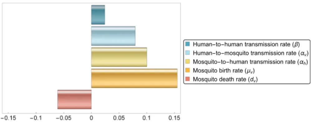
In Sect.4, we study the global stability of the disease-free equilibrium in the case ofR0 < 1 the persistence of the disease in case ofR0 > 1. We also calculate the basic reproduction number of the time-constant variant of the model. In Sect.5, we present a case study for two South American countries. We estimate the parameter values for both countries and perform sensitivity analysis to determine the parameters which have the largest effect on the outcome of the epidemic. We provide numerical simulations to study the possible effects of an alteration of various parameters to see what kind of changes might lead to an annual recurrence of the disease. The paper is closed by a discussion.
2 Mathematical Model
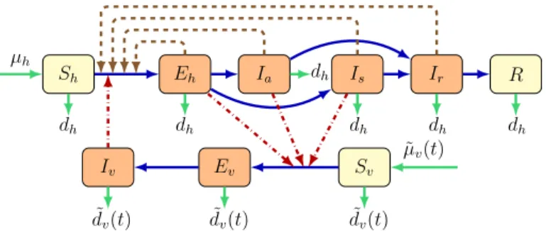
We divide the total human population into six compartments: susceptible Sh(t), exposedEh(t), symptomatically infectedIs(t), asymptomatically infectedIa(t), con- valescentIr(t), and recoveredR(t)at timet >0, while the vector population is divided into three classes: susceptibleSv(t), exposedEv(t), and infectiousIv(t)individuals.
The total human population Nh(t)and the total mosquito population Nv(t)are given by:
Nh(t)=Sh(t)+Eh(t)+Ia(t)+Is(t)+Ir(t)+R(t), Nv(t)=Sv(t)+Ev(t)+Iv(t).
Our model takes the form
Sh(t)= μh−βτeEh(t)+τaIa(t)+Is(t)+τrIr(t)
Nh(t) Sh(t)−dhSh(t)
−α˜h(t)
Nh(t)Iv(t)Sh(t),
Eh(t)= βτeEh(t)+τaIa(t)+Is(t)+τrIr(t)
Nh(t) Sh(t)+ α˜h(t)
Nh(t)Iv(t)Sh(t)
−νhEh(t)−dhEh(t),
Ia(t)= qνhEh(t)−γaIa(t)−dhIa(t), Is(t)= (1−q)νhEh(t)−γsIs(t)−dhIs(t),
Ir(t)= γaIa(t)+γsIs(t)−γrIr(t)−dhIr(t), R(t)= γrIr(t)−dhR(t),
Sv(t)= ˜μv(t)− ˜αv(t)ηeEh(t)+ηaIa(t)+Is(t)
Nh(t) Sv(t)− ˜dv(t)Sv(t), Ev(t)= ˜αv(t)ηeEh(t)+ηaIa(t)+Is(t)
Nh(t) Sv(t)−νvEv(t)− ˜dv(t)Ev(t),
Iv(t)= νvEv(t)− ˜dv(t)Iv(t), (1)
where μ˜v(t), α˜h(t),α˜v(t)and d˜v(t)denote mosquito birth rate, transmission rate from an infectious mosquito to a susceptible human, the transmission rate from infected humans to susceptible mosquitoes and mosquito death rate, respectively. In our model, we assumedμ˜v(t),α˜h(t),α˜v(t)andd˜v(t)to be continuous, positiveω- periodic functions. An individual may progress from susceptible (Sh) to exposed (Eh) upon contracting the disease. An exposed individual moves either to the symptomat- ically infected class Is or to the asymptomatically infected class Ia, depending on whether that person shows symptoms or not. Infected people with or without symp- toms move to the convalescent compartment Ir including those who have already recovered, but who can still transmit the disease via sexual contact. After the conva- lescent period, one moves to the recovered compartmentR. Mosquitoes may progress from susceptible (Sv) to exposed (Ev) and then to infectious (Iv) class. The description of the model parameters is summarized in Table1, while the transmission diagram of the model can be seen in Fig. 1. We note that although the population is non-constant, the recruitment term in our model is given asμh instead ofμhNh, as the countries studied in this work can be expected to be close to constant within a reasonable time interval. Doing so, we also followed among others the works Bacaër and Guernaoui (2006), Liu et al. (2010), Qu et al. (2017), Wang et al. (2013). We emphasize that a similar model was established and studied in Dénes et al. (2019), which also included differentiation of the two sexes. However, no stability analysis was performed in that paper, only numerical results were presented.
Fig. 1 (Color figure online) Zika virus dynamics spread including vectorial and sexual transmission. Brown nodes are infectious and yellow nodes are non-infectious. Blue solid arrows show the progression of infec- tion, while brown dashed arrows show direction of human-to-human transmission and red dash-dotted arrows show direction of transmission between humans and mosquitoes. Green arrows show birth and death
Table 1 Description of parameters of model1
Parameter Description
μh Human birth rate
dh Human death rate
β Transmission rate from infected humans to susceptible humans αh Baseline value of transmission rate from mosquitoes to humans αv Baseline value of transmission rate from humans to mosquitoes q Proportion of asymptomatic infections
τe, τa, τr Relative human-to-human transmissibility of (exposed, asymptomatic and convalescent) humans to symptomatic humans
ηe, ηa Relative human-to-mosquito transmissibility of (exposed and asymptomatically infected) humans to symptomatically infected humans
γa Progression rate fromIatoIr γs Progression rate fromIstoIr γr Recovery rate of convalescent humans
νh Human incubation rate
νv Mosquitoes incubation rate
μv Baseline value of mosquito birth rate dv Baseline value of mosquito death rate
We defineXh =(Sh,Eh,Ia,Is,Ir,R)and the functionsg1,g2,g3∈C(R6+,R+) by
g1(Xh)=
0, ifXh=(0,0,0,0,0,0),
τeEh+τaIa+Is+τrIr
Sh+Eh+Ia+Is+Ir+RSh, ifXh∈R6+\ {(0,0,0,0,0,0)}, g2(Xh)=
0, ifXh=(0,0,0,0,0,0),
1
Sh+Eh+Ia+Is+Ir+RSh, ifXh∈R6+\ {(0,0,0,0,0,0)}, g3(Xh)=
0, ifXh=(0,0,0,0,0,0),
ηeEh(t)+ηaIa(t)+Is(t)
Sh+Eh+Ia+Is+Ir+R, ifXh∈R6+\ {(0,0,0,0,0,0)}.
(2)
Clearly,g1(Xh),g2(Xh)andg3(Xh)are continuous onR6+. Also,g1(Xh),g2(Xh)and g3(Xh)are globally Lipschitz onR6+. By a change of variableNh=Sh+Eh+Ia+ Is+Ir +Rand from (2), system (1) is equivalent to
Sh(t)=μh−βg1(Sh,Eh,Ia,Is,Ir,Nh)− ˜αh(t)g2(Sh,Eh,Ia,Is,Ir,Nh)Iv(t)
−dhSh(t),
Eh(t)=βg1(Sh,Eh,Ia,Is,Ir,Nh)+ ˜αh(t)g2(Sh,Eh,Ia,Is,Ir,Nh)Iv(t)
−νhEh(t)−dhEh(t),
Ia(t)=qνhEh(t)−γaIa(t)−dhIa(t), Is(t)=(1−q)νhEh(t)−γsIs(t)−dhIs(t),
Ir(t)=γaIa(t)+γsIs(t)−γrIr(t)−dhIr(t), Nh(t)=μh−dhNh(t),
Sv(t)= ˜μv(t)− ˜αv(t)g3(Sh,Eh,Ia,Is,Ir,Nh)Sv(t)− ˜dv(t)Sv(t), Ev(t)= ˜αv(t)g3(Sh,Eh,Ia,Is,Ir,Nh)Sv(t)−νvEv(t)− ˜dv(t)Ev(t),
Iv(t)=νvEv(t)− ˜dv(t)Iv(t). (3)
We now prove the existence of a disease-free periodic solution of (3). For the human subsystem of system (3) with initial condition
X0=(Sh(0),Eh(0),Ia(0),Is(0),Ir(0),Nh(0),Sv(0),Ev(0),Iv(0))∈R9+, we have the linear differential equation
dNh
dt (t)=μh−dhNh(t). (4)
One can easily see that (4) has a single equilibrium Nh∗ = μdhh, which is globally asymptotically stable andNh(t)is bounded.
To determine the disease-free periodic solution of (3), we study equation
Sv(t)= ˜μv(t)− ˜dv(t)Sv(t), (5) with initial valueSv(0)∈R+. Equation (5) has a single positiveω-periodic solution Sv∗(t), globally attractive inR+and thus, system (3) has a single disease-free periodic solutionE0=
Nh∗,0,0,0,0,Nh∗,Sv∗(t),0,0 .
To formulate our next result, we introduce the notationshL =supt∈[0,ω)h(t)and hM =inft∈[0,ω)h(t)for a continuous, positiveω-periodic functionh(t).
Lemma 1 There exists an Nv∗ = μd˜˜LvL
v > 0such that every forward solution in X :=
(Sh,Eh,Ia,Is,Ir,Nh,Sv,Ev,Iv)∈R9+:Nh ≥Sh+Eh+Ia+Is+Ir, Nv
≥Sv+Ev+Iv
of(3)eventually enters
GN∗ := {(Sh,Eh,Ia,Is,Ir,Nh,Sv,Ev,Iv)∈X :Nh
≤ Nh∗, Sv+Ev+Iv≤ Nv∗<∞ ,
and for each Nv(t)≥Nv∗, GNis positively invariant for (3). Further, it holds that
t→+∞lim
Nv(t)−S∗v(t)
=0, where Nv(t)=Sv(t)+Ev(t)+Iv(t).
Proof From (3), for the mosquito subsystem, we have
Nv(t)= ˜μv(t)− ˜dv(t)Nv(t)≤μLv −dvMNv(t)≤0, ifNv(t)≥Nv∗,
which implies thatGN,Nv(t)≥ Nv∗, is forward invariant and eventually, every positive orbit will enterGN∗. For the second part of the proof, let us assume that
y(t)=Nv(t)−Sv∗(t), t≥0. We then have that
y(t)= − ˜dv(t)y(t), which implies that
t→+∞lim y(t)=0. Hence, the proof is complete.
3 Basic Reproduction Number, Local Stability
Following the technique and the notations introduced by Wang and Zhao (2008), we show the local stability of the disease-free periodic equilibriumE0of (3) for appropri- ate parameter values. First, we introduce the basic reproduction numberR0for system (3). LetX =(Eh,Ia,Is,Ir,Ev,Iv,Sh,Nh,Sv)T withF(t,X(t)),V+(t,X(t)) andV−(t,X(t))denote the input rate of newly infected individuals, the input rate of individuals by other means and the rate of transfer of individuals out of compartments, respectively.
System (3) is equivalent to
X(t)=F(t,X(t))−V(t,X(t)), (6) whereV(t,X(t))=V−(t,X(t))−V+(t,X(t)). We know that (6) has the disease- free periodic solutionX∗(t)=
0,0,0,0,0,0,Nh∗,Nh∗,Sv∗(t)
.Then by a simple computation we obtain
F(t)=
⎡
⎢⎢
⎢⎢
⎢⎢
⎣
βτe βτa β βτr 0α˜h(t)
0 0 0 0 0 0
0 0 0 0 0 0
0 0 0 0 0 0
ηeα˜v(t)
Nh∗ Sv∗(t) ηaαN˜v∗(t)
h S∗v(t) α˜Nv(∗t)
h Sv∗(t) 0 0 0
0 0 0 0 0 0
⎤
⎥⎥
⎥⎥
⎥⎥
⎦ ,
V(t)=
⎡
⎢⎢
⎢⎢
⎢⎢
⎣
νh+dh 0 0 0 0 0
−qνh γa+dh 0 0 0 0
−(1−q)νh 0 γs+dh 0 0 0
0 −γa −γs γr +dh 0 0
0 0 0 0 νv+ ˜dv(t) 0
0 0 0 0 −νv d˜v(t)
⎤
⎥⎥
⎥⎥
⎥⎥
⎦ ,
M(t)=
⎡
⎣−dh 0 0 0 −dh 0 0 0 − ˜dv(t)
⎤
⎦. (7)
Furthermore, F(t)is non-negative, and−V(t)is cooperative. Also F(t)−V(t)is irreducible for all t. It is straightforward to see that the conditions (A1)–(A6) are satisfied, andX∗(t)is linearly asymptotically stable in the disease-free subspace
Xs =(0,0,0,0,0,0,Sh,Nh,Sv)∈R9+.
AssumeY(t,s),t≥sis the evolution operator of the linearω-periodic system dy
dt = −V(t)y. (8)
That is, for eachs∈R, the 6×6 matrixY(t,s)satisfies d
dtY(t,s)= −V(t)Y(t,s), ∀t≥s, Y(s,s)=I,
where I is the 6×6 identity matrix. Thus, the monodromy matrixΦ−V(t)of (8) is equal toY(t,0), t≥0. Therefore, the condition (A7) holds.
Supposeφ(s),ω-periodic ins, is the initial distribution of infectious individuals.
ThenF(s)φ(s)gives us the rate of new infections produced by the infected individuals introduced at times. Givent ≥ s, thenY(t,s)F(s)φ(s)supplies the distribution of those newly infected at times who remain in the infected compartments at timet.
Then ψ(t):=
t
−∞Y(t,s)F(s)φ(s)ds= ∞
0
Y(t,t−a)F(t−a)φ(t−a)da,
is the distribution of accumulative new infections at timetdue to all infected individ- ualsφ(s)introduced at time less thant.
We denote byCωthe ordered Banach space ofω-periodic functions fromRtoR6, equipped with the maximum norm · ∞and introduce the positive cone
Cω+:= {φ∈Cω:φ(t)≥0, ∀t∈R}.
Following Wang and Zhao (2008), we then define the linear operatorL:Cω →Cω as
(Lφ)(t)= ∞
0
Y(t,t−a)F(t−a)φ(t−a)da, ∀t ∈R, φ∈Cω, (9) called the next infection operator. The basic reproduction number of (1) is defined as R0:=ρ(L), i.e. the spectral radius of the next infection operatorL.
For the periodic case, letW(t, λ)be the monodromy matrix of dω
dt =
−V(t)+1 λF(t)
ω, t ∈R,
with parameter λ ∈ (0,∞). Since F(t)is non-negative and−V(t)is cooperative, we obtain that ρ(W(ω, λ)) is continuous and non-increasing in λ ∈ (0,∞) and limλ→∞ρ(W(ω, λ)) <1.
From the above discussion, we obtain the following result for the local asymptotic stability of the disease free periodic solutionE0of our model (1).
Theorem 1 (Wang and Zhao (2008, Theorem 2.1))The following statements hold.
(i) Ifρ(W(ω, λ))=1has a positive solutionλ0, thenλ0is an eigenvalue of operator L, and henceR0>0.
(ii) IfR0>0, thenλ=R0is the unique solution ofρ(W(ω, λ))=1.
(iii) R0=0if and only ifρ(W(ω, λ)) <1for allλ >0.
Theorem 2 (Wang and Zhao (Wang and Zhao (2008), Theorem 2.2))The following statements hold.
(i) R0=1if and only ifρ(ΦF−V(ω))=1;
(ii) R0>1if and only ifρ(ΦF−V(ω)) >1;
(iii) R0<1if and only ifρ(ΦF−V(ω)) <1.
Hence, the disease-free periodic solutionE0is locally asymptotically stable ifR0<1, and unstable ifR0>1.
3.1 Derivation of the Basic Reproduction Number of the Autonomous Model To calculate the basic reproduction ratioR0Aof the autonomous model obtained from (3) by setting the time-dependent parameters (mosquito birth (μ˜v(t)≡μv) and death rates (d˜v(t)≡dv) and biting rates (α˜h(t)≡αhandα˜v(t)≡αv) to constant, we follow the general approach established by Diekmann et al. (2009).
Substituting the values in the disease-free equilibriumSv∗=μdvv in equation (7), for allt≥0, we obtain the JacobianFgiven by
F=
⎡
⎢⎢
⎢⎢
⎢⎢
⎣
βτe βτa β βτr 0αh
0 0 0 0 0 0
0 0 0 0 0 0
0 0 0 0 0 0
ηeαvμvdh
μhdv ηaαvμvdh
μhdv αvμvdh
μhdv 0 0 0
0 0 0 0 0 0
⎤
⎥⎥
⎥⎥
⎥⎥
⎦ ,
and the JacobianV given by
V =
⎡
⎢⎢
⎢⎢
⎢⎢
⎣
νh+dh 0 0 0 0 0
−qνh γa+dh 0 0 0 0
−(1−q)νh 0 γs+dh 0 0 0
0 −γa −γs γr +dh 0 0
0 0 0 0 νv+dv 0
0 0 0 0 −νv dv
⎤
⎥⎥
⎥⎥
⎥⎥
⎦ ,
therefore the characteristic polynomial of the next generation matrixF V−1is λ4
λ2−Rhhλ−RhvRvh
=0, (10)
where Rhh = β
dh+νh
τe+ qτaνh
γa+dh +(1−q)νh
γs+dh + τrνh(γs(γa+dh)+q(γa−γs)dh) (γa+dh)(γr+dh)(γs +dh)
, Rhv= αvdhμv
dvμh(dh+νh)
ηe+ qηaνh
γa+dh +(1−q)νh
γs+dh
, Rvh= αhνv
dv(dv+νv).
The characteristic polynomial therefore is the quadratic equation
λ2−Rhhλ−RhvRvh=0. (11)
According to Diekmann et al. (2009), the basic reproduction number is the spectral radius ofF V−1. Thus, the basic reproduction number corresponds to the dominant eigenvalue given by the root of the quadratic equation (11)
R0A=Rhh+
Rhh2 +4RhvRvh
2 , (12)
whereRhhandRv=RhvRvhare the basic reproduction numbers corresponding to sexual transmission and vector-borne transmission, respectively. From (12), we found thatRhh+Rv<1 is the necessary and sufficient condition forR0A<1.
4 Threshold Dynamics
Here we study the global stability of the disease-free equilibrium of model (3) and the persistence of the infectious compartments. We use the general theory for the extinction or persistence of infectious given by Rebelo et al. (2011) to show that if the basic reproduction ratioR0is less than 1, then the unique disease-free equilibrium X∗(t)=
0,0,0,0,0,0,Nh∗,Nh∗,Sv∗(t)
is globally asymptotically stable (G.A.S.)
and the disease dies out, while if the basic reproduction ratioR0 is larger than 1, the disease persists. Moreover, we follow Zhang and Zhao (2007), Liu et al. (2010), Nakata and Kuniya (2010) and Qu et al. (2017) to prove the existence of a positive periodic solution of (3) ifR0>1.
4.1 Global Stability of the Disease-Free Equilibrium
In this subsection, we use the general method given by Rebelo et al. (2011) to show that the disease-free equilibrium is G.A.S. ifR0<1.
Theorem 3 IfR0<1, then the disease-free periodic solutionX∗(t)of system(6)is globally asymptotically stable and ifR0>1, then it is unstable.
Proof By Theorem2, we know thatX∗(t)is unstable ifR0>1 and ifR0<1, then X∗(t)is locally asymptotically stable. According to the above discussion in Sect.3, the conditions (A1) to (A7) in Rebelo et al. (2011) are satisfied.
MoreoverX∗(t)=
0,0,0,0,0,0,Nh∗,Nh∗,Sv∗(t)
is the unique periodic solution in the set of the disease-free statesXs.
Clearly,S(t)≤ Nh(t), for allt ≥0. From Lemma1, for any >0, there exists t() >0 such thatSv(t)≤ Nv(t)≤ Sv∗(t)+for allt ≥t().
Substituting into system (3), we obtain
Eh(t)≤β (τeEh(t)+τaIa(t)+Is(t)+τrIr(t))+ ˜αh(t)Iv(t)−(νh+dh)Eh(t), Ia(t)≤qνhEh(t)−γaIa(t)−dhIa(t),
Is(t)≤(1−q)νhEh(t)−γsIs(t)−dhIs(t), Ir(t)≤γaIa(t)+γsIs(t)−γrIr(t)−dhIr(t), Ev(t)≤ ˜αv(t)ηeEh(t)+ηaIa(t)+Is(t)
Nh∗
Sv∗(t)+ε
−(νv+ ˜dv(t))Ev(t), Iv(t)≤νvEv(t)− ˜dv(t)Iv(t),
for allt ≥t().
Setμ():=min{Sv∗(·)/
Sv∗(·)+
}. Then we have the following system:
dU˜(t) dt ≤
F(t) μ()−V(t)
U˜(t), ∀t ≥t(), (13)
whereU(t)˜ =
E˜h(t),I˜a(t),I˜s(t),I˜r(t),E˜v(t),I˜v(t)
. ThenU(t)˜ → 0 ast → ∞ and the disease dies out.
By applying the first part of (Rebelo et al.2011, Theorem 2), we conclude that the disease-free periodic solutionX∗(t)is G.A.S. since it is G.A.S. inXs.
4.2 Persistence of the Infective Compartments
In this subsection, we will show that the infectives are persistent ifR0>1, by using the general method given by Rebelo et al. (2011).
Theorem 4 IfR0>1then system(3)is persistent with respect to Eh, Ia, Is, Ir, Ev and Iv.
Proof Persistence of Eh+Ia+Is implies persistence of Eh,Ia andIs, and hence, persistence ofIr,EvandIv. If there exists >0 such that lim inft→+∞
Eh+Ia+ Is
≥, thenEh≥ 3−Ia−Isfor larget. Thus, from system (3), we obtain
Ia ≥qνh
3 −(qνh+γa+dh)Ia−qνhIs, Is≥(1−q)νh
3 −((1−q)νh+γs +dh)Is−(1−q)νhIa. (14) Thus, we have
Ia(t)≥ 3
qνh
qνh+γa+dh =:κa(), Is(t)≥
3
(1−q)νh
(1−q)νh+γs +dh =:κs().
(15)
By introducing the inequality (15) into the fifth equation of system (3), we get Ir≥γaκa()+γsκs()−(γr +dh)Ir, (16) and hence,
Ir(t)≥ γaκa()+γsκs()
γr+dh =:κr(). (17)
ConsiderEh≤,Ia≤,Is ≤,Ir ≤,R≤,Ev≤andIv≤for allt≥t0. There existst1≥t0such that|Nh(t)−Sh∗| ≤and|Nv(t)−Sv∗(t)| ≤for allt≥t1. Therefore,Sh(t)= Nh(t)−Eh(t)−Ia(t)−Is(t)−Ir(t)−R(t)≥ S∗h−5 and Sv(t)=Nv(t)−Ev(t)−Iv(t)≥Sv∗(t)−3for allt≥t1. From the equation forEv of system (3), we have
Ev ≥ ˜αv(t)ηe
3+(ηa−ηe)Ia+(1−ηe)Is
Nh∗ (Sv∗(t)−3)−(νv+ ˜dv(t))Ev.(18) By (Rebelo et al.2011, Lemma 1), we obtain that
Ev(t)≥ α˜vM ηe
3+(ηa−ηe)κa()+(1−ηe)κs()
(S∗vM(t)−3)
2Nh∗(νv+ ˜dvL) =:κe().(19)
Substituting the inequality (19) into the equation forIvof system (3), we obtain Iv ≥νvκe()− ˜dv(t)Iv, (20) and again by (Rebelo et al.2011, Lemma 1), we have
Iv(t)≥ νvκe()
2d˜vL =:Kv(). (21)
Setλ():=max{1/ 1− N5∗
h
,max
Sv∗(·)/(Sv∗(·)−3
)}.From the equations of system (3), for sufficiently larget ≥t1, we obtain
Eh(t)≥β
τeEh(t)+τaIa(t)+Is(t)+τrIr(t)+ ˜αh(t)Iv(t) 1−N5∗ h
−(νh+dh)Eh(t)
≥β
τeEh(t)+τaIa(t)+Is(t)+τrIr(t)+ ˜αh(t)Iv(t) 1
λ()−(νh+dh)Eh(t), Ia(t)≥qνhEh(t)−γaIa(t)−dhIa(t),
Is(t)≥(1−q)νhEh(t)−γsIs(t)−dhIs(t), Ir(t)≥γaIa(t)+γsIs(t)−γrIr(t)−dhIr(t), Ev(t)≥ ˜αv(t)
ηeEh(t)+ηaIa(t)+Is(t) SvN∗(∗t) h −N3∗
h
−(νv+ ˜dv(t))Ev(t)
≥ ˜αv(t)
ηeEh(t)+ηaIa(t)+Is(t)Sv∗(t)
λ() −(νv+ ˜dv(t))Ev(t), Iv(t)≥νvEv(t)− ˜dv(t)Iv(t).
From Lemma1, it is clear that condition (A8) in Rebelo et al. (2011) is satisfied. There- fore, the assumptions of (Rebelo et al.2011, Theorem 4) are satisfied and system (3) is persistent with respect toEh,Ia,Is,Ir,Ev, andIv.
4.3 Existence of Positive Periodic Solutions
Define X :=
(Sh,Eh,Ia,Is,Ir,Nh,Sv,Ev,Iv)∈R9+ , X0:=
(Sh,Eh,Ia,Is,Ir,Nh,Sv,Ev,Iv)∈R+×Int(R4+)×R2+×Int(R2+) ,
and
∂X0:=X\X0= {(Sh,Eh,Ia,Is,Ir,Nh,Sv,Ev,Iv):EhIaIsIrEvIv=0}. LetP:R9+→R9+be the Poincaré map associated with (3), that is,
P(x0)=u(ω,x0), forx0∈R9+,
whereu(t,x0)is the unique solution of (3) withu(0,x0)=x0. It is easy to see that Pm(x0)=u(mω,x0), ∀m≥0.
Letd(x,y)denote Euclidean distance inR9. The following lemma is analogous with (Liu et al.2010, Lemma 3.1).
Lemma 2 IfR0 > 1, then there exists aσ∗ > 0 such that for any x0 ∈ X0, with x0−E0 ≤σ∗we have
lim sup
m→∞ d
Pm(x0),E0
≥σ∗.
Proof By Theorem2, we have thatρ(ΦF−V(ω)) >1 ifR0>1.Then, we can choose η >0 small enough such thatρ(ΦF−V−Mη(ω)) >1 where
Mη(t)=
⎡
⎢⎢
⎢⎢
⎢⎢
⎣
0 0 0 0 0 0
0 0 0 0 0 0
0 0 0 0 0 0
0 0 0 0 0 0
2η
Nh∗+ηηeα˜v(t) N2∗η
h+ηηaα˜v(t) N2∗η
h+ηα˜v(t)0 0 0
0 0 0 0 0 0
⎤
⎥⎥
⎥⎥
⎥⎥
⎦ .
The equation dSdth =μh−dhShhas a unique equilibriumSh∗=Nh∗which is a global attractor inR+.
The perturbed system dSˆh(t)
dt =(μh−βσ1− ˜αh(t)σ2)−dhSˆh(t), (22) has a unique solution
Sˆh(t, σ1, σ2)=e−dht
Sˆh(0, σ1, σ2)+ t
0
e−dhs(μh−βσ1−αh(s)σ2)ds
,
through any initial valueSˆh(0, σ1, σ2), and it has a unique periodic solution Sˆh∗(t, σ1, σ2)=e−dht
Sˆh∗(0, σ1, σ2)+ t
0
e−dhs(μh−βσ1−αh(s)σ2)ds
,
where
Sˆ∗h(0, σ1, σ2)= ω
0 e−dhs(μh−βσ1−αh(s)σ2)ds e−dhω−1 .