AmathematicalmodelforLassafevertransmissiondynamicsinaseasonalenvironmentwithaviewtothe2017–20epidemicinNigeria NonlinearAnalysis:RealWorldApplications

(1)

Contents lists available atScienceDirect

Nonlinear Analysis: Real World Applications

www.elsevier.com/locate/nonrwa

A mathematical model for Lassa fever transmission dynamics in a seasonal environment with a view to the 2017–20 epidemic in Nigeria

Mahmoud A. Ibrahim

^a^,^b^,^∗

, Attila Dénes

^a

aBolyai Institute, University of Szeged, Aradi vértanúk tere 1., Szeged, H-6720, Hungary

bDepartment of Mathematics, Faculty of Science, Mansoura University, Mansoura 35516, Egypt

a r t i c l e i n f o

Article history:

Received 23 June 2020

Received in revised form 7 February 2021

Accepted 9 February 2021 Available online xxxx Keywords:

Lassa haemorrhagic fever Periodic epidemic model Basic reproduction number Global stability

Uniform persistence

a b s t r a c t

In this paper, we formulate and study a compartmental model for Lassa fever transmission dynamics considering human-to-human, rodent-to-human transmission and the vertical transmission of the virus in rodents. To incorporate the impact of periodicity of weather on the spread of Lassa, we introduce a non- autonomous model with time-dependent parameters for rodent birth rate and carrying capacity of the environment with respect to rodents. We introduce the basic reproduction number and show that it can be used as a threshold parameter concerning the global dynamics. It also shown that the disease-free periodic solution is globally asymptotically stable in the case of R₀ <1 and if R₀ >1, then the disease persists. We show numerical studies for the Lassa fever in Nigeria and give examples to describe what kind of parameter changes might trigger the periodic recurrence of Lassa fever.

1. Introduction

Lassa haemorrhagic fever (LHF), or Lassa fever for short is a zoonotic, acute viral hemorrhagic fever caused by the Lassa virus from theArenaviridae family [1]. The disease was first described in the 1950s, though the virus causing it was only identified in 1969 [2]. The disease was named after the Nigerian town Lassa, where the first cases were observed. LHF is usually transmitted to humans via direct or indirect exposure to food or other items contaminated with urine or feces of infected multimammate rats (Mastomys natalensis), through the respiratory or gastrointestinal tracts. Person-to-person transmission has also been observed [3]. The virus remains in body fluids even after recovery: in urine for 3–9 weeks from infection and for three months in male genital secretions [3]. Lassa fever is endemic among rats in parts of West Africa, while it is endemic in humans in several countries of the region. In these regions, the number of infections

∗ Corresponding author at: Bolyai Institute, University of Szeged, Aradi v´ertan´uk tere 1., Szeged, H-6720, Hungary.

E-mail address: mibrahim@math.u-szeged.hu(M.A. Ibrahim).

https://doi.org/10.1016/j.nonrwa.2021.103310

(2)

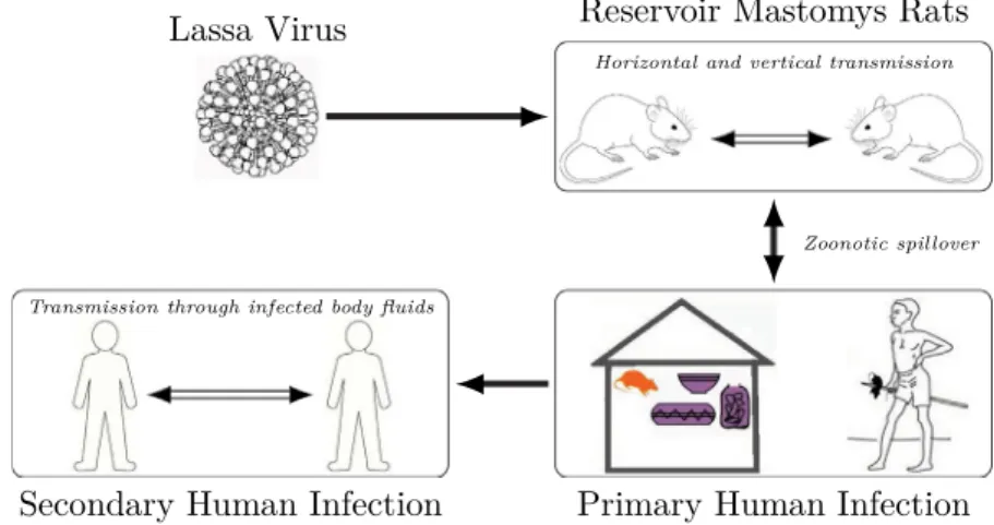
Fig. 1. Lassa fever transmission. The figure shows modes of transmission (human-to-human, human-to-rodent, rodent-to-human and rodent-to-rodent).

per year is estimated between 100,000 and 300,000, with around 5000 deaths. Lassa menaces mostly those who live in rural areas where multimammate rats are present, especially where poor sanitation and crowded living conditions are typical.Fig. 1shows the possible methods of LHF transmission.

About 80% of people infected with Lassa fever have only mild or no symptoms. Symptom onset occurs usually 1–3 weeks after exposure, these include fever, tiredness, weakness, and headache. 20% of infected develop a severe multisystem disease with symptoms including bleeding gums, respiratory distress, vomiting, chest, back and abdomen pain, facial swelling, low blood pressure. Neurological problems can also be observed, such as hear loss, tremors, encephalitis. Approximately 1% of infections result in death due to multi-organ failure. However, the disease is particularly severe in women in the third trimester of their pregnancy, with high rates of maternal death (29%) observed, while an estimated 80%–95% fetal and neonatal mortality is reported [1,4,5].

Treatment of Lassa fever includes antiviral medication, fluid replacement and blood transfusions. For women in late pregnancy, inducing delivery is necessary.

Although Lassa fever appears in WHO’s Blueprint list of diseases to be prioritized for research and development [6], compared with other infectious diseases, a relatively small number of mathematical modelling studies have been published up to now. Onah et al. [7] extended anSIR–SI-type compartmental model by introducing different control intervention measures, e.g. external protection, treatment, isolation and rodent control. They used optimal control theory to determine how to reduce disease transmission with minimal cost. Musa et al. [8] established a model describing the interaction between humans and rodents including quarantine, isolation and hospitalization. The authors showed the presence of a forward bifurcation with a stability switch between the disease-free and the endemic equilibrium. Also, they fitted the model to data from 2016–19 to find that initial susceptibility increased across the three outbreaks in these years.

Zhao et al. [9] studied the epidemiological features of Lassa epidemics in various regions of Nigeria. They assessed the connection between the reproduction number and rainfall. They determined the infectivity of Lassa by the reproduction number estimated from four types of growth models. They fitted the models to Lassa surveillance data and estimated the reproduction number in various regions. Akhmetzanov et al. [10]

applied a model to study the datasets of human infection, population changes of rodents as well as weather changes to quantify the seasonal drivers of Lassa fever transmission. They obtained that seasonal migration of rats plays a key role in regulating the periodicity of Lassa epidemics. The peak exposure of humans to rats is shortly after the beginning of the dry season and correlates with the mating period of rodents.

Although some of the above works put an emphasis on the time-changing nature of Lassa transmission dynamics, so far, no compartmental model with time-dependent parameters has been established. In

(3)

this work, we set up and study a compartmental epidemic model for Lassa fever transmission dynamics considering infected humans with mild or severe symptoms, treatment, human-to-human and rodent-to human transmission as well as time-dependent parameters. Namely, modelling the annual periodic change of weather, we introduce time-periodic parameters for rodent birth rate and carrying capacity of the environment with respect to rodents. To study the dynamics of our time-periodic model, we will apply the theory initiated in [11–15], later applied in several periodic epidemic models (see, e.g. [16–23]). Here we adapt these methods to our system with human-to-human and rodent-to-human transmission with a logistic growth of rodents.

The rest of the paper is structured as follows. In the next section we introduce the time-dependent mathematical model for Lassa fever transmission dynamics. In Section 3 we study the existence of the disease-free periodic solution. In Section4 we calculate the basic reproduction number of our model using various methods. In Section5, we show that depending on the basic reproduction number, either the disease- free periodic solution is globally asymptotically stable or the disease persists in the population. In Section6 we provide numerical simulations for both scenarios supporting the theoretical results.

2. Seasonal model for Lassa fever transmission

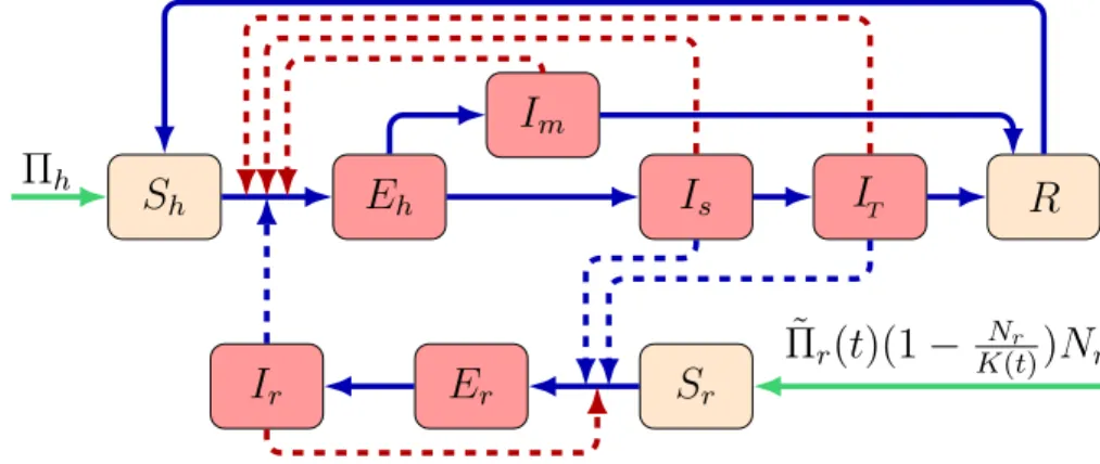
We divide the human population into six compartments: susceptibleS_h(t), exposedE_h(t), symptomatically infectedIs(t), mildly infectedIm(t), treatedIT(t), and recovered individuals with temporary immunity R(t). The total size of the human population at any timetis denoted by

N_h(t) =S_h(t) +E_h(t) +I_m(t) +I_s(t) +I_T(t) +R(t).

An individual may proceed from susceptible (Sh) to exposed (Eh) upon contracting the disease. Individuals in the exposed compartment have no symptoms yet. After the incubation time, an exposed individual moves either to the symptomatically infected class (I_s) or to the mildly infected class (I_m), depending on whether that person shows symptoms or not. Infected people fromIs may move to the treated compartment (IT), including those who need hospital treatment. After the infection period, recovered persons move to the class R.

Fig. 2. Schematic diagram of the LHF transmission among rodents and humans. Red nodes denote infectious, brown nodes denote non-infectious states. Blue solid arrows demonstrate infection progress, while red dashed arrows represent direction of human-to-human transmission and rodent-to-rodent transmission. Blue dashed arrows show direction of transmission between humans and rodents. Green arrows show recruitment rate for humans and maximum growth rate of the rodents. (For interpretation of the references to colour in this figure legend, the reader is referred to the web version of this article.)

The vector population (Mastomys natalensis rat) at time t, denoted by Nr(t), is divided into three compartments: susceptibleS_r(t), exposedE_r(t) and infectiousI_r(t), respectively. Thus

Nr(t) =Sr(t) +Er(t) +Ir(t).

3

(4)

Table 1

Description of parameters of model(1).

Parameters Description

Πh Recruitment rate for humans

d Natural death rates of humans

δs, δT Disease-induced death rates for humans βm, βs, βT Transmission rates from human-to-human

βhr Transmission rate from human-to-rodent

β_rh Transmission rate from rodent-to-human

β_r Transmission rate from rodent-to-rodent

η_s, η_T Relative transmissibility of infectious human-to-rodent

θ Proportion of mild infections

γs Progression rate fromIs toIT

γm, γT Recovery rates

νh Humans incubation rate

ν_r Rodents incubation rate

ξ Rate of relapse fromRtoS_h

K_r Average carrying capacity of the environment for the rodents

Π_r Baseline value of rodents birth rate

µ Natural death rates of rodents

b Phase angle (month of peak in seasonal forcing)

Λ Amplitude of seasonality

The transmission dynamics is shown in the flow diagram (seeFig. 2) and our model takes the form dSh(t)

dt =Π_h−βmIm(t) +βsIs(t) +βTIT(t)

N_h(t) S_h(t)−β_rh Ir(t)

N_h(t)S_h(t)−dS_h(t) +ξR(t), dEh(t)

dt = βmIm(t) +βsIs(t) +βTIT(t)

N_h(t) Sh(t) +βrh

Ir(t)

N_h(t)Sh(t)−νhEh(t)−dEh(t), dIm(t)

dt =θνhEh(t)−γmIm(t)−dIm(t), dIs(t)

dt = (1−θ)νhEh(t)−γsIs(t)−(d+δs)Is(t), dIT(t)

dt =γsIs(t)−γTIT(t)−(d+δT)IT(t), dR(t)

dt =γmIm(t) +γTIT(t)−ξR(t)−dR(t), dS_r(t)

dt = ˜Π_r(t) (

1−N_r(t) K(t)

)

N_r(t)−β_hrη_sI_s(t) +η_TI_T(t)

Nh(t) S_r(t)−β_r I_r(t)

Nr(t)S_r(t)−µS_r(t), dE_r(t)

dt =β_hrη_sI_s(t) +η_TI_T(t)

Nh(t) S_r(t) +β_rI_r(t)

Nr(t)S_r(t)−ν_rE_r(t)−µE_r(t), dIr(t)

dt =νrEr(t)−µIr(t),

(1)

where ˜Π_r(t) andK(t) denote the time-dependent per capita birth rate and maximal carrying capacity of theMastomys natalensisrats. In our model we assumed ˜Πr(t) andK(t) are continuous, positiveω-periodic functions. We denote byΠh anddthe human birth and death rate, respectively. There is also an additional disease-induced death rate, denoted byδ_sandδ_T for those in the compartmentsI_sandI_T, respectively. The description of the model parameters are summarized inTable 1.

3. The disease-free periodic solution

3.1. Existence of the disease-freeω-periodic solution

In this section, we study the existence and uniqueness of the disease-free periodic solution of system(1).

Define

(5)

ϕ=(

S_h(0), E_h(0), I_m(0), I_s(0), I_T(0), R(0), S_r(0), E_r(0), I_r(0))

∈R⁹+.

In case of no disease, for the total human populationN_hwith a positive initial conditionϕ∈R⁹+, we have the equation

dNh(t)

dt =Πh−dNh(t), (2)

from which we obtain

Nh(t) =Nh(0)e^−dt+Πh

d (1−e^−dt). (3)

with an arbitrary initial value Nh(0). Eq. (3) has a unique equilibrium N_h^∗ = ^Π_d^h in R+. Consequently,

|Nh(t)−N_h^∗| →0 ast→ ∞andN_h^∗ is globally attractive onR+. To identify the disease-free periodic solution of(1), consider

dS_r(t)

dt = ˜Π_r(t) (

1−S_r(t) K(t) )

S_r(t)−µS_r(t), (4)

with initial conditionS_r(0)∈R+. Eq. (4)has a unique positiveω-periodic solution

S_r^∗(t) = e

∫t

0( ˜Π_r(s)−µ)ds

∫t 0

Π˜_r(τ) K(τ)e

∫τ

0( ˜Π_r(s)−µ)ds

dτ+

∫ω 0

Πr(τ)˜ K(τ)e

∫τ

0( ˜Πr(s)−µ)ds dτ e

∫ω

0 ( ˜Πr(s)−µ)ds

−1

>0, (5)

which is globally attractive in R+. Thus, system (1) has a unique disease-free periodic solution E0 = (S_h^∗,0,0,0,0,0, S_r^∗(t),0,0)

, whereS_h^∗= ^Π_d^h.

Lemma 3.1. There is N_r^∗ = lim sup_t→∞^{K(t)( ˜}_Π_˜^Π^r^(t)−µ)

r(t) > 0 such that any forward solution in R⁹+ of (1) enters eventually

Ω_N^∗

r :={

(Sh, Eh, Im, Is, IT, R, Sr, Er, Ir)∈R⁹+:Nh⩽N_h^∗, Nr⩽N_r^∗} , and for eachN_r(t)⩾N_r^∗,Ω_N is a positively invariant set w.r.t.(1). Further, it holds that

t→+∞lim (Nr(t)−S^∗_r(t)) = 0.

Proof. From(1), we have dNr(t)

dt = ˜Πr(t) (

1−Nr(t) K(t)

)

Nr(t)−µNr(t)

⩽ (

Π˜r(t)−µ−Π˜r(t) K(t)Nr(t)

)

Nr(t)⩽0 ifNr(t)⩾N_r^∗,

which implies thatΩN, Nr(t)⩾N_r^∗, is positively invariant and each forward orbit entersΩN^∗ eventually.

For the second part of the proof, let us assume thatz(t) =Nr(t)−S_r^∗(t), t⩾0. Then, it follows that dz(t)

dt =−µz(t), which implies that lim_t→+∞z(t) = 0. □

5

(6)

4. Basic reproduction numbers and local stability

Based on the method established by Wang and Zhao [14], we demonstrate the local stability of the disease-free periodic equilibriumE₀ of(1)in terms of the basic reproduction numberR₀.

Linearizing the system(1)atE₀, we obtain the equations for exposed and infectious human and rodent populations, respectively:

dEh(t)

dt = βmIm(t) +βsIs(t) +βTIT(t)

N_h^∗ S_h^∗−βrh

Ir(t)

N_h^∗ S_h^∗−(νh+d)Eh(t), dI_m(t)

dt =θν_hE_h(t)−γ_mI_m(t)−dI_m(t), dI_s(t)

dt = (1−θ)ν_hE_h(t)−γ_sI_s(t)−(d+δ_s)I_s(t), dI_T(t)

dt =γ_sI_s(t)−γ_TI_T(t)−(d+δ_T)I_T(t), dE_r(t)

dt =βhr

η_sI_s(t) +η_TI_T(t)

N_h^∗ S_r^∗(t) +βr

I_r(t)

N_r^∗ S_r^∗(t)−(νr+µ)Er(t), dIr(t)

dt =νrEr(t)−µIr(t).

Let us introduce the matrix functionsF(t) andV(t) of dimension 7×7 as

F(t) =

⎡

⎢

⎣

0βm S∗

h N∗ h

βs S∗

h N∗ h

β_T^S

∗ h N∗ h

0 β_rh^S

∗ h N∗ h

0 0 0 0 0 0

0 0 βhr^ηs N∗

h

S^∗_r(t)βhr^ηT N∗

h

S^∗_r(t) 0β_r^S

∗r(t) N∗

r

0 0 0 0 0 0

⎤

⎥

⎦ ,

V(t) =

⎡

⎢

⎣

ν_h+d 0 0 0 0 0

−θν_h γ_m+d 0 0 0 0

−(1−θ)ν_h 0 γ_s+d+δ_s 0 0 0

0 0 −γs γ_T+d+δ_T 0 0

0 0 0 0 νr+µ0

0 0 0 0 −νr µ

⎤

⎥

⎦. Note thatF(t) is a non-negative matrix function, while−V(t) is cooperative.

SupposeZ(t, s), t⩾s, is the evolution operator of the linear system dy

dt =−V(t)y. (6)

Thus, fors∈R,Z(t, s) satisfies the equation dZ(t, s)

dt = −V(t)Z(t, s), ∀t⩾s, Z(s, s) =I, whereI stands for the 6×6 identity matrix.

Assumeϕ(s) is the initial distribution of infected,ω-periodic ins. Then,F(s)ϕ(s) provides the rate of new cases due to those infected who were introduced at times. Fort⩾s, the termZ(t, s)F(s)ϕ(s) provides us the distribution of the infectious individuals who newly became infected at timesand who are still infected at timet. Therefore,

ψ(t) :=

∫ t

−∞

Z(t, s)F(s)ϕ(s)ds=

∫ ∞ 0

Z(t, t−a)F(t−a)ϕ(t−a)da,

gives the distribution of accumulative new infections attgenerated by all infectedϕ(s) who were introduced at any times⩽t.

(7)

Let us assume thatC_ω is the ordered Banach space ofω-periodic functions fromRtoR⁶, endowed with the usual maximum norm∥ · ∥_∞ and introduce the positive cone

C_ω⁺:={ϕ∈C_ω:ϕ(t)⩾0, ∀t∈R}.

Define the linear next infection operatorL:Cω→Cωby (Lϕ)(t) =

∫ ∞ 0

Z(t, t−a)F(t−a)ϕ(t−a)da, ∀t∈R, ϕ∈C_ω. (7) Then, the basic reproduction number of(1)isR0:=ρ(L), the spectral radius ofL [14].

LetW(t, λ) be the monodromy matrix of the linear ω-periodic equation dw

dt = (

−V(t) + 1 λF(t)

)

w, ∀t∈R, with parameterλ∈(0,∞).

To numerically approximate the basic reproduction number, we will apply the following theorem from [14].

Theorem 4.1([14, Theorem 2.1]).The following statements are valid.

(i) Ifρ(W(ω, λ)) = 1has a positive solutionλ0, thenλ0 is an eigenvalue of operatorL, and henceR0>0.

(ii) IfR0>0, thenλ=R0is the unique solution of ρ(W(ω, λ)) = 1.

(iii) R₀= 0 if and only ifρ(W(ω, λ))<1for allλ >0.

4.1. Local stability of the disease-free periodic solution

First we recall the following theorem from [14].

Theorem 4.2([14, Theorem 2.2]).The following statements are valid:

(i) R0= 1 if and only ifρ(Φ_F−V(ω)) = 1.

(ii) R₀>1 if and only ifρ(Φ_F−V(ω))>1.

(iii) R0<1 if and only ifρ(Φ_F−V(ω))<1.

As per the above discussion, the following theorem concerns the local stability of the disease-free periodic solutionE0 of(1).

Theorem 4.3. The disease-free periodic solutionE₀of(1)is locally asymptotically stable ifR₀<1, whereas it is unstable ifR0>1.

Proof . The Jacobian matrix of(1)calculated atE₀is given by.

J(t) =[_F(t)−V_{(t) 0}

A(t) M

] , where

A(t) = [₀_β

m βs β_T 0β_rh

0 0 0 0 0 0

0 0 βhr^ηs N∗

h

S_r^∗(t)βhr^ηT N∗

h

S_r^∗(t) 0 βr

]

and M =

[_−d _ξ ₀

0 −ξ−d 0

0 0 −µ

] .

According to [24], E0 is LAS if ρ(ΦM(ω)) < 1 and ρ(ΦF−V(ω)) < 1. M is a constant matrix and its eigenvalues areλ₁=−d <0,λ₂=−ξ−d <0 andλ₃=−µ <0. Sinceλ₁,λ₂andλ₃are negative, we have ρ(Φ_M) <1. Consequently, the stability ofE₀ depends on ρ(Φ_F−V(ω)). Thus, E₀ is locally asymptotically stable if ρ(Φ_F−V(ω)) < 1, and unstable if ρ(Φ_F−V(ω)) > 1. Hence, we complete the proof by applying Theorem 4.2. □

7

(8)

4.2. The time-average basic reproduction number

Using the general method introduced in [25], we calculate the basic reproduction number of the autonomous model obtain from (1) by setting the time-varying parameters ˜Π_r(t) ≡ Π_r and K(t) ≡ K_r to constant.

Substituting the value ofS_r^∗(t)≡S_r^∗=K_r(Πr−µ Πr

)in the disease-free equilibrium for allt⩾0, we obtain the JacobianF given by

F =

⎡

⎢

⎣

0βm βs β_T 0β_rh

0 0 0 0 0 0

0 0 βhr^ηs N∗ h

S^∗_r βhr^ηT N∗

h S_r^∗0 βr

0 0 0 0 0 0

⎤

⎥

⎦, and the JacobianV given by

V =

⎡

⎢

⎣

ν_h+d 0 0 0 0 0

−θν_h γ_m+d 0 0 0 0

−(1−θ)ν_h 0 γs+d+δs 0 0 0

0 0 −γs γ_T+d+δ_T 0 0

0 0 0 0 ν_r+µ0

0 0 0 0 −νr µ

⎤

⎥

⎦, thus the characteristic polynomial ofF V⁻¹ is

λ⁴(

λ²−(Rhh+Rrr)λ+RhhRrr− RhrRrh

)= 0, (8)

where

Rhh= νh

d+ν_h

( θβm

γ_m+d+ (1−θ)βs

γ_s+d+δ_s+ (1−θ)γsβT

(γ_s+d+δ_s)(γ_T +d+δ_T) )

, Rhr= (1−θ)ν_hβ_hrS_r^∗

Π_h

d (γs+d+δs)(d+νh) (

η_s+ γ_sη_T γT +d+δT

) , R_rh= βrhνr

µ(µ+νr), R_rr = βrνr

µ(µ+ν_r).

The characteristic polynomial therefore is the quadratic equation

λ²−(Rhh+Rrr)λ+RhhRrr− RhrRrh= 0. (9) According to [25], the basic reproduction number is the largest absolute eigenvalue ofF V⁻¹ and therefore, it is given by the root of the quadratic equation(9),

R^A₀ =ρ(F V⁻¹) =Rhh+Rrr+

√

(Rhh− Rrr)² + 4R²_v

2 , (10)

where Rhh, Rrr and Rv = √

RhrRrh are the basic reproduction numbers of human-to-human transmission, rodent-to-rodent transmission and vectorial transmission, respectively. From (10) one can see that

R_hh+R_rr+R²_v

R_hhRrr+1 >1 is the necessary and sufficient condition forR^A₀ >1.

To calculate the time-average basic reproduction number, [R0], of the associated non-autonomous system, we use the following remark.

Remark 4.4. For a continuousω-periodic functiong(t), define its average (using the notation presented in [26]) as

[g] := 1 ω

∫ ω 0

g(t)dt.

(9)

Then, the time-average basic reproduction number is given by [R0] = Rhh+Rrr+

√

(Rhh− Rrr

)2

+ 4[Rhr]Rrh

2 , (11)

where

[Rhr] = (1−θ)ν_hβ_hr[S_r^∗]

Π_h

d (γ_s+d+δ_s)(d+ν_h) (

η_s+ γ_sη_T γT +d+δT

) , [S_r^∗] = [K]

([ ˜Πr]−µ [ ˜Πr]

) . 5. Threshold dynamics

In this section, we show the dynamics of our model depending on the basic reproduction number. We prove the existence of a positive periodic solution of model(1)if the basic reproduction numberR0>1. In this case, the disease persists, whereas if the basic reproduction numberR₀<1, then the unique disease-free equilibriumE₀ is globally asymptotically stable and the disease goes extinct.

We will need the following lemma to show the global stability ofE₀and the persistence of the disease.

Lemma 5.1([15, Lemma 2.1]). Letµ= _ω¹lnρ(Φ_A(·)(ω)). Then there exists a positive, ω-periodic function v(t)such thate^µtv(t)is a positive solution ofx^′ =A(t)x.

5.1. Global stability of the disease-free equilibrium

Theorem 5.2. If R0<1, then the disease-free periodic solutionE0 of(1)is globally asymptotically stable and ifR0>1, then it is unstable.

Proof . We realize fromTheorem 4.3 that ifR0>1, thenE₀is unstable and ifR0<1, thenE₀is locally asymptotically stable. Consequently, it remains only to show that forR0<1,E₀ is globally attractive. For anyε₁, fromLemma 3.1and Eq.(2), there existsT₁>0 such thatS_r(t)⩽S_r^∗(t) +ε₁, N_r(t)⩾S^∗_r(t)−ε₁ andN_h(t)⩾N_h^∗−ε₁ fort > T₁. Thus, we get

Sh(t)

N_h(t)⩽ S_h^∗

N_h^∗−ε₁, Sr(t)

N_h(t)⩽ S_r^∗+ε1

N_h^∗−ε₁ and Sr(t)

N_r(t)⩽ S^∗_r+ε1

N_r^∗(t)−ε₁. From(1), we obtain

dE_h(t) dt ⩽(

βmIm(t) +βsIs(t) +βTIT(t)−βrhIr(t)) S_h^∗ N_h^∗−ε1

−(νh+d)Eh(t), dIm(t)

dt =θνhEh(t)−γmIm(t)−dIm(t), dIs(t)

dt = (1−θ)ν_hE_h(t)−γ_sI_s(t)−(d+δ_s)I_s(t), dIT(t)

dt =γ_sI_s(t)−γ_TI_T(t)−(d+δ_T)I_T(t), dR(t)

dt =γ_mI_m(t) +γ_TI_T(t)−ξR(t)−dR(t), dE_r(t)

dt ⩽β_hr(

η_sI_s(t) +η_TI_T(t))S^∗_r(t) +ε₁ N_h^∗−ε1

+β_rI_r(t)S^∗_r(t) +ε₁ N_r^∗−ε1

−(ν_r+µ)E_r(t), dIr(t)

dt =νrEr(t)−µIr(t),

9

(10)

fort > T₁. LetM_ε₁(t) be the 6×6 matrix function defined by

⎡

⎢

⎣

−ν_h−d β_m ^S

∗ h N∗

h−ε1 β_s ^S

∗ h N∗

h−ε1 β_T ^S

∗ h N∗

h−ε1 0 β_rh ^S

∗ h N∗

h−ε1

θν_h −γm−d 0 0 0 0

(1−θ)ν_h 0 −γs−d−δs 0 0 0

0 0 γ_s −γ_T−d−δ_T 0 0

0 0 βhrηsS∗

r+ε1 N∗

h−ε1 βhrη_T^S r∗+ε1 N∗

h−ε1 −νr−µ βr S∗ r+ε1 N∗

r(t)−ε1

0 0 0 0 νr −µ

⎤

⎥

⎦ .

Consider the following auxiliary system:

d ˜U(t)

dt =Mε₁(t) ˜U(t), (12)

where ˜U(t) =(E˜_h(t),I˜_m(t),I˜_s(t),I˜_T(t),E˜_r(t),I˜_r(t)) .

Applying Theorem 4.2, it flows that R0 < 1 if and only if ρ(ΦF−V(ω)) < 1. It is obvious that limε₁→0ΦM_ε₁(ω) =Φ_F−V(ω). Asρ(Φ_F−V(ω)) is continuous, we can chooseε1>0 small enough such that ρ(ΦM_ε

1(ω))<1.

FromLemma 5.1, there is an ω-periodic positive function p₁(t) such that p₁(t)e^ξ¹^t is a solution of(12) andξ₁= _ω¹lnρ(Φ_M_ε

1(ω))<0. For anyh(0)∈R⁶+, we can choosen^∗>0 s.t.h(0)⩽n^∗p₁(0) where h(t) = (Eh(t), Im(t), Is(t), IT(t), Er(t), Ir(t))^T.

Applying the comparison principle [27, Theorem B.1], we obtainh(t)⩽p1(t)e^ξ¹^tfor allt >0. Therefore, we get

t→∞lim (Eh(t), Im(t), Is(t), IT(t), Er(t), Ir(t))^T = (0,0,0,0,0,0)^T.

One can easily find thatNh(t)→N_h^∗ as t→ ∞. Let ε1>0, we can findtε₁ >0 such that Im(t)⩽ε1 and IT(t)⩽ε1for allt⩾tε₁. Then, the equation forR^′(t) of(1)gives ^dR(t)_dt ⩽(γm+γT)ε1−ξR(t)−dR(t), for larget. From whereR(t)→0 ast→+∞. Thus, from(5) and the first equation of(1), we obtain that

t→∞lim S_h(t) =S_h^∗ and lim

t→∞S_r(t) =S_r^∗(t), and the proof is complete. □

5.2. Existence of positive periodic solutions

Define

X := {

(Sh, Eh, Im, Is, IT, R, Sr, Er, Ir)∈R⁹+

}, X₀:=

{

(Sh, Eh, Im, Is, IT, R, Sr, Er, Ir)∈X :Eh>0, Im>0, Is>0, I_T >0, E_r>0, I_r>0

} , and

∂X₀:=X\X₀.

LetP:R⁹+→R⁹+ denote the Poincar´e map corresponding to(1), then P is given by P(x⁰) =u(ω, x⁰), forx⁰∈R⁹+,

whereu(t, x⁰) is the unique solution of(1)with initial conditionx⁰∈X. Clearly, P^m(x⁰) =u(mω, x⁰), ∀m⩾0.

(11)

Proposition 5.3. The sets X₀ and∂X₀are both positively invariant w.r.t. the flow defined by(1).

Proof . Letϕ∈X₀ be any initial condition. By solving(1)for allt >0, we get that S_h(t) =e

∫t

0−(a₁(s)+d)ds[

S_h(0) +∫t 0

(Π_h+ξR(t)) e

∫s

0(a₁(r)+d)dr

ds ]

>0, (13)

Eh(t) =e^−(ν^h^+d)t[

Eh(0) +∫t

0a1(s)Sh(s)e^(νⁿ^+d)sds]

>0, (14)

I_m(t) =e^−(γ^m^+d)t[

I_m(0) +θν_h∫t

0E_h(s)e^(γ^m^+d)sds]

>0, (15)

Is(t) =e^−(γ^m^+d+δ^s^)t[

Im(0) + (1−θ)νh∫t

0Eh(s)e^(γ^m^+d+δ^s^)sds]

>0, (16)

I_T(t) =e^−(γ^T^+d+δ^T^)t[

I_T(0) +γ_s∫t

0I_s(r)e^(γ^T^+d+δ^T^)rdr]

>0, (17)

Rh(t) =e^−(ξ+d)t[

R(0) +∫t

0(γsIs(r) +γTIT(r))e^(ξ+d)rdr]

>0, (18)

S_r(t) =e

∫t

0−(a₂(s)+µ)ds[

S_r(0) +∫t 0Π˜_r(s)(

1−^N_K(s)^r^(s)) N_r(s)e

∫s

0(a₂(r)+µ)dr

ds ]

>0 (19) E_r(t) =e^−(ν^r^+µ)t[

E_r(0) +∫t

0a₂(s)S_r(s)e^(ν^r^+µ)sds]

>0, (20)

Ir(t) =e^−µt[

Ir(0) +νr

∫t

0Er(s)e^−µsds]

>0, (21)

where

a₁(t) =βmIm(t) +βsIs(t) +βTIT(t)

N_h(t) +β_rhIr(t) N_h(t), a2(t) =βhr

ηsIs(t) +ηTIT(t) N_h(t) +βr

Ir(t) N_r(t).

Thus,X0is a positively invariant set. SinceX is also positively invariant and∂X0 is relatively closed inX, it gives∂X0 is positively invariant. □

Lemma 5.4. IfR0>1, then there exists aσ >0 such that for anyϕ∈X0with∥ϕ−E0∥⩽σ, we have lim sup

m→∞

d(P^m(ϕ), E0)⩾σ.

Proof . We recognize from Theorem 4.2that ρ(Φ_F−V(ω))>1 if R0 >1. Then, we can selectκ >0 small enough such that we haveρ(Φ_F−V_−M_κ(ω))>1, whereM_κ(t) is the 6×6 matrix function defined by

⎡

⎣

0β_mκ β_sκ β_Tκ 0β_rhκ

0 0 0 0 0 0

0 0 βhrη_sκ βhrη_Tκ0 β_rκ

0 0 0 0 0 0

⎤

⎦.

Using the continuous dependence of the solutions on initial values, we find aσ=σ(κ)>0 such that for allϕ∈X₀ with∥ϕ−E₀∥⩽σ, it holds that

∥u(t, ϕ)−u(t, E0)∥⩽κ, for 0⩽t⩽ω.

We further claim that

lim sup

m→∞

d(P^m(ϕ), E₀)⩾σ. (22)

By contradiction suppose that(22)does not hold. Then lim sup

m→∞

d(P^m(ϕ), E0)< σ, (23)

11

(12)

for someϕ∈X₀. Without loss of generality, we may assume d(P^m(ϕ), E₀)< σ, ∀m≥0.

Then, from the above discussion, we have that

∥u(t, P^m(ϕ)−u(t, E₀))∥< σ, ∀m≥0, t∈[0, ω].

For anyt⩾0, lett=mω+t1, wheret1∈[0, ω) andm= [_ω^t], which is the largest integer less than or equal to _ω^t. Then, we get

∥u(t, ϕ)−u(t, E₀)∥=∥u(t₁, P^m(ϕ))−u(t₁, E₀)∥< σ, for allt⩾0, which implies that

Sh(t) N_h(t) ⩾ S_h^∗

N_h^∗ −κ, Sr(t) N_h(t) ⩾ S_r^∗

N_h^∗ −κ and Sr(t)

N_r(t) ⩾S_r^∗(t) N_r^∗ −κ.

Then for∥ϕ−E0∥⩽σ, we obtain dEh(t)

dt ⩾ (βmIm(t) +βsIs(t) +βTIT(t)−βrhIr(t)) (S^∗_h

N_h^∗ −κ )

−(νh+d)Eh(t), dI_m(t)

dt =θν_hE_h(t)−γ_mI_m(t)−dI_m(t), dI_s(t)

dt = (1−θ)ν_hE_h(t)−γ_sI_s(t)−(d+δ_s)I_s(t), dI_T(t)

dt =γ_sI_s(t)−γ_TI_T(t)−(d+δ_T)I_T(t), dEr(t)

dt ⩾βhr(ηsIs(t) +ηTIT(t)) (S_r^∗

N_h^∗ −κ )

+βrIr(t) (S_r^∗

N_r^∗ −κ )

−(νr+µ)Er(t), dI_r(t)

dt =ν_rE_r(t)−µI_r(t).

Next we consider the auxiliary linear system d ˆU(t)

dt =(

F(t)−V(t)−M_κ(t))U(t),ˆ (24)

where ˆU(t) =(Eˆ_h(t),Iˆ_m(t),Iˆ_s(t),Iˆ_T(t),Eˆ_r(t),Iˆ_r(t)) .

Now we have thatρ(Φ_F−V_−M_κ(ω)) > 1. Again, we have from Lemma 5.1 that there exists a positive, ω-periodic functionp₂(t) such that h(t) =e^ξ²^tp₂(t) is a solution of(24)andξ₂=_ω¹ lnρ(Φ_F−V_+M_κ(ω))>0.