http://www.aimspress.com/journal/MBE
DOI: 10.3934/mbe.2019225 Received: 31 December 2018 Accepted: 09 May 2019 Published: 21 May 2019
Research article
The e ff ect of the needle exchange program on the spread of some sexually transmitted diseases
Eliza B´anhegyi1, Attila D´enes1,∗, J´anos Karsai1and L´aszl´o Sz´ekely1,2
1 Bolyai Institute, University of Szeged, Aradi v´ertan´uk tere 1., H-6720 Szeged, Hungary
2 Department of Mathematics, Institute of Environmental Engineering Systems, Szent Istv´an University, P´ater K´aroly utca 1., H-2100 G¨od¨oll˝o, Hungary
* Correspondence: Email: denesa@math.u-szeged.hu; Tel:+3662343883; Fax:+3662544548.
Abstract: In this paper we consider a model for the spread of a sexually transmitted disease considering sexual transmission and spread via infected needles among intravenous drug users. Besides the transmission among drug users, we also consider sexual contacts between intravenous drug users and non-drug users. Furthermore, the needles are considered as a vector population. For several European countries, a sharp increase of sexually transmitted diseases was reported and several others are rated as endangered based on the number of syringes given out per intravenous drug users per year. The main purpose of the paper is to investigate the dynamics of this model including the effect of needle exchange and study the risk of an increased transmission among non-drug users, induced by the reduction of the needle exchange program. Following the determination of the basic reproduction number R0 it is shown that all solutions tend to the unique disease-free equilibrium if R0 < 1. We also prove that the disease persists in the human population ifR0 > 1. Our numerical simulations, based on real life and hypothetical data for HIV, suggest that a decrease in the rate of the distribution and discharge rate of new needles might imply that the considered disease is becoming endemic in the considered human population of drug users and non-drug users. A variant of our model with time- variable needle distribition parameter is fitted to recent HIV data from Hungary to give a forecast for the number of infected in the following years.
Keywords: compartmental model; sexually transmitted diseases; needle exchange program; global stability; uniform persistence
1. Introduction
Besides their principal transmission form, some sexually transmitted diseases (STD) can also be spread via several other ways, including donor tissue, blood, breastfeeding or during childbirth. In
this paper we shall focus on STDs which can be transmitted among intravenous drug users (IDU) through sharing syringes or needles during drug use. Typical examples for pathogens spread this way are human immunodeficiency virus (HIV), hepatitis B, C, D virus, as well as the bacteriumTreponema pallidumcausing syphilis [1, 2, 3, 4]. At the same time, some IDUs also engage in high-risk sexual behaviour facilitating the transmission of these diseases between different groups [5, 6]. Hence, the application of infected needles not only elevates the risk of transmission among IDUs, but also creates a greater risk for non-drug users.
Recently, the European Centre for Disease Prevention and Control reported a sharp increase of HIV notifications in Greece and Romania due to the reduction of the sterile needle exchange program among drug users [7]. Several other European countries – Belgium, Cyprus, Hungary, Slovakia, Turkey – were rated as endangered based on the number of syringes given out per IDU per year.
Several studies have already been published on STDs with the possibility of transmission via blood [9, 10, 11, 8]. In [9] and [8], the authors considered different compartments for people with different rates of addiction to intravenous drugs. Here we enhance the models developed by Kaplan et al. [12, 13, 14]. In these works, the authors established models to examine the dynamics of the population of susceptible and contaminated needles as well. Based on these models, further research was carried out by Greenhalgh et al. [15, 16, 17]. Several papers deal with a special subgroup of the population, e.g. people visiting shooting galleries [18] or a rare transmission way, e.g. parental exposure and blood transfusion [19]. Ji et al. [11] studied optimal needle allocation to prevent HIV transmission.
Motivated by the above reports and predictions, our main purpose is to investigate the dynamics of a model including the effect of needle exchange and study the risk of an increased transmission among non-drug users, induced by the reduction of the needle exchange program. Our new approach to this problem consists in considering not just a needle population and the prevalence of infections among drug users, but beyond the latter one, a population of sexually active humans consisting of drug users and non-drug users.
The structure of the paper is the following. In the next section, we establish a system of differential equations to model the spread of a disease through sexual contact and needle sharing. In Section 3, we calculate the disease-free equilibrium and the basic reproduction numberR0. In Section 4, we show that the disease-free equilibrium is globally asymptotically stable ifR0 <1. In Section 5, we show that the infected compartments are uniformly persistent ifR0 >1.
In Section 6, we provide some numerical simulations which suggest that the reduction of the needle exchange program can highly contribute to the spread of diseases both among drug users and non-drug users. We fit a time-dependent variant of our model to recent data from Hungary to give a prognosis for the expected number of infections in the next decade.
2. The model
We establish a compartmental model, in which, besides humans, also needles are considered as a population. In our model, the human population is divided into four isolated groups: S denotes susceptible individuals who do not use drugs,SD stands for susceptible IDUs. We denote byI those who are infected and do not use drugs, while ID stands for infected IDUs. The needle population is separated to two disjoint classes,SN denotes susceptible, clean needles, while IN stands for infected
needles. As in a developed country more than 99% of the cases happen via sexual transmission or contaminated needles, in our paper we concern only these two major factors, and investigate a model emphasizing their role (see e.g. [20]).
We assume that both human and needle populations are closed in the sense that birth and death rates (denoted byλ) are balanced (S +SD+I+ID = const., SN +IN = const.) and that the disease spread by people-people or people-needles contacts.
The transitions between the compartments are as follows. All newborn individuals enter the S compartment. Susceptibles become addicted to intravenous drugs and hence move from the compartmentS to SD with rate a. The other way around, g denotes the rate of giving up drug use.
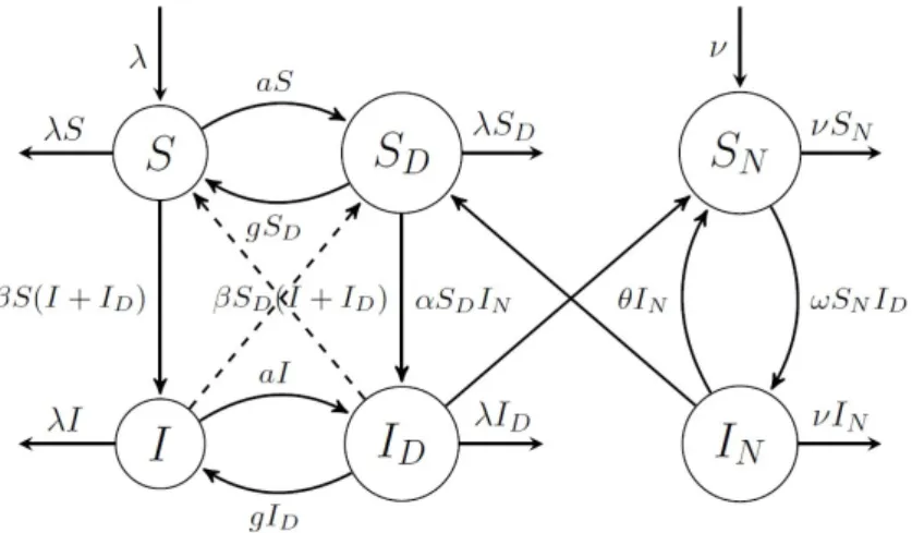
Getting addicted to and giving up drugs is modelled similarly for the infected compartmentsI andID. The model includes two ways of contracting HIV. Sexual intercourse with an infected partner results in getting infected with a rate β. The other way of infection considered in our model is the use of contaminated needles among IDUs. We consider a needle population where new needles are distributed with a constant rateν, and we assume that old needles are discarded with the same rateν. Transmission rate from infected drug users to clean needles is denoted by ω, while α denotes the transmission rate from infected needles to susceptible drug users. Used needles are sterilized with rate θ. The transmission diagram of the model is shown in Figure 1.
Figure 1. HIV spread in the population.
Using the above notations and assumptions, we obtain the following system of ordinary differential equations:
S0(t)=λ−(a+λ)S(t)+gSD(t)−βS(t)(I(t)+ID(t)), I0(t)= −(a+λ)I(t)+gID(t)+βS(t)(I(t)+ID(t)),
S0D(t)=aS(t)−(g+λ)SD(t)−βSD(t)(I(t)+ID(t))−αSD(t)IN(t), ID0(t)=aI(t)−(g+λ)ID(t)+βSD(t)(I(t)+ID(t))+αSD(t)IN(t), S0N(t)=ν−νSN(t)+θIN(t)−ωSN(t)ID(t),
IN0(t)= −(ν+θ)IN(t)+ωSN(t)ID(t).
(2.1)
3. Disease-free equilibrium and basic reproduction number
In this section, we study the disease-free equilibrium which can be obtained by solving the following algebraic system of equations:
0=λ−S(λ+a)+gSD−βS(I+ID),
0=−SD(λ+g)−αSDIN+aS −βSD(I+ID), 0=ν−νSN+θIN−ωSNID.
The unique disease-free equilibrium can be calculated as E0 = g+λ
a+g+λ,0, a
a+g+λ,0,1,0
! .
The most important parameter to characterize an epidemic is the basic reproduction number R0 defined as the expected number of secondary infections caused by a single infectious individual over the course of his/her infectious period, introduced in a completely susceptible population.
We apply the method of next generation matrices introduced by Diekmann, Heesterbeek and Roberts [22]. According to this method, the basic reproduction number is given by the dominant eigenvalue of the next generation matrix −FV−1, where F is the transmission matrix and V is the transition matrix of the infection subsystem at the disease-free equilibrium. In our case, this subsystem is given by
I0(t)= −(a+λ)I(t)+gID(t)+βS(t)(I(t)+ID(t)),
ID0(t)=aI(t)−(g+λ)ID(t)+βSD(t)(I(t)+ID(t))+αSD(t)IN(t), IN0(t)= −(ν+θ)IN(t)+ωSN(t)ID(t),
hence, the transmission and transition matrices are F =
β(g+λ)
a+g+λ β(g+λ) a+g+λ 0
aβ a+g+λ
aβ
a+g+λ aα a+g+λ
0 ω 0
(3.1) and
−V =
a+λ −g 0
−a g+λ 0
0 0 ν+θ
. (3.2)
Therefore, the next generation matrix is calculated as
NGM=−FV−1 =
β(g+λ) λ(a+g+λ)
β(g+λ)
λ(a+g+λ) 0
aβ λ(a+g+λ)
aβ
λ(a+g+λ) aα (ν+θ)(a+g+λ) λ(aaω+g+λ)
ω(a+λ)
λ(a+g+λ) 0
.
The characteristic equation of the next generation matrix has the form χ(x)= −x3+ β
λx2+ aαω(a+λ)
λ(a+g+λ)2(θ+ν)x− aαβω(g+λ)
λ(a+g+λ)3(θ+ν) =0.
Remark 3.1. It is easy to see that there are three distinct real eigenvalues, two positive and one negative. Observe the cubic Vieta’s formulas:
x1+x2+x3 = β λ,
x1x2+x1x3+x2x3 =− aαω(a+λ) λ(a+g+λ)2(θ+ν), x1x2x3 =− aαβω(g+λ)
λ(a+g+λ)3(θ+ν).
Let us suppose that x1 = R0 and x2,x3 are complex conjugate roots. The productR0x2x3 is negative according to the third equation, which leads to a contradiction, since multiplying R0 by a complex conjugate pair is always positive. Moreover, the product of three real roots will be negative only if the number of the negative terms is odd.
Using Cardano’s formula for cubic equations we obtain
R0= 3λβ +
β3
27λ3 −2λ(aaαβ(g+λ)ω
+g+λ)3(θ+ν) +6λ2aαβ(a(a+g++λ)λ)ω2(θ+ν) − r β3
27λ3−2λ(aaαβ(g+λ)ω
+g+λ)3(θ+ν) +6λ2aαβ(a(a+g++λ)λ)ω2(θ+ν)
2
+
−9λβ22−3λ(aaα(a+λ)ω
+g+λ)2(θ+ν)
3
1/3
+
β3
27λ3−2λ(aaαβ(g+λ)ω
+g+λ)3(θ+ν) +6λ2aαβ(a(a+g++λ)λ)ω2(θ+ν) + r
β3
27λ3 −2λ(aaαβ(g+λ)ω
+g+λ)3(θ+ν)+6λ2(aaαβ(a+g++λ)λ)ω2(θ+ν)
2
+
−9λβ22 −3λ(aaα(a+λ)ω
+g+λ)2(θ+ν)
3
1/3
.
The formula forR0is far too complicated to be easily applicable in the analysis. In order to cope with this difficulty, we introduce the parameterP0as follows:
P0= χ(1)= β
λ+ aαω(a+λ)
λ(a+g+λ)2(θ+ν) − aαβω(g+λ)
λ(a+g+λ)3(θ+ν) −1. (3.3) Although this expression is much simpler, one can see that the parameterP0is not equivalent toR0as a threshold parameter: the smaller positive eigenvalue may pass through 1 as well. It is easy to see that R0 <1 impliesP0< 0 andP0 >0 impliesR0 >1 (see Figure 2).
P0
R0
-0.5 0.5 1.0 1.5x
-0.4 -0.2 0.2 0.4χ(x)
P0
R0
-0.5 0.5 1.0 1.5x
-0.4 -0.2 0.2 0.4χ(x)
Figure 2. R0 <1 impliesP0< 0 andP0 >0 impliesR0 >1.
4. Global asymptotic stability of the disease-free equilibrium
In this section, we will show that the basic reproduction number calculated in the previous section serves as a threshold parameter regarding the dynamics of our system. We need to show some simple assertions before we can state the main theorem of the section. Let f: [0,∞) → R. We introduce the notations
f∞ Blim sup
t→∞
f(t) and f∞ Blim inf
t→∞ f(t).
for the limit superior, resp. the limit inferior of f ast→ ∞.
Lemma 4.1. For the limit superior of S,SD,SN the following inequalities hold:
S∞ ≤ g+λ
a+g+λ, S∞D ≤ a
a+g+λ, S∞N ≤1.
Proof. Adding the first two equations of (2.1), we obtain
(S(t)+I(t))0 = λ−(a+λ) (S(t)+I(t))+g(SD(t)+ID(t)). Since 1−SD(t)−ID(t)=S(t)+I(t) we get
(S(t)+I(t))0+(a+g+λ) (S(t)+I(t))= λ+g.
According to the fluctuation lemma (see e.g. [28]), we have (a+g+λ) (S +I)∞ =g+λ,
(S +I)∞ = g+λ a+g+λ. SinceS andI are nonnegative,S∞ ≤ (S +I)∞ holds.
Similarly, let us consider (SD(t)+ID(t))0:
(SD(t)+ID(t))0= a(S(t)+I(t))−(g+λ)(SD(t)+ID(t)), from which we have
(SD(t)+ID(t))0+(a+g+λ)(SD(t)+ID(t))=a(S(t)+I(t)+SD(t)+ID(t)).
SinceS(t)+I(t)+SD(t)+ID(t)=1 we get
(SD(t)+ID(t))0+(a+g+λ)(SD(t)+ID(t))= a.
Using the fluctuation lemma we obtain
(SD+ID)∞= a a+g+λ. SinceSDandIDare nonnegative,S∞D ≤(SD+ID)∞holds.
S∞N ≤1 holds trivially.
In the proof of the global asymptotic stability of the disease-free equilbrium E0 we will need [27, Theorem 2.1]. In order to apply this result, we first recall this theorem.
Theorem A([27, Theorem 2.1]). Let us consider a system x0 =F(x,y)− V(x,y),
y0 =g(x,y) (4.1)
with g = (g1, . . . ,gm)T. The vectors x = (x1, . . . ,xn) ∈ Rn and y = (y1, . . . ,ym)T ∈ Rm stand for the populations in the disease compartments and the non-disease compartments, respectively. The functionsF andV are defined as F = (F1, . . . ,Fn)T and V = (V1, . . . ,Vn)T such thatFi denotes the rate of new infections in theith disease compartment andVi, i= 1, . . . ,ndenote transition terms.
We assume that the disease-free systemy0 = g(0,y) has a unique equilibrium y0 > 0 which is locally asymptotically stable within the disease-free space. Let us define the twon×nmatricesF andV as
F = ∂Fi
∂xj
(0,y0)
!
and V = ∂Vi
∂xj
(0,y0)
!
and let
f(x,y)B(F−V)x− F(x,y)+V(x,y).
LetωT ≥0 be the left eigenvector of the matrixV−1Fcorresponding to the eigenvalueR0. If f(x,y)≤0 inΓ⊂ Rn++m, F ≥0,V−1 ≥0 andR0 ≤1, thenQ=ωTV−1xis a Lyapunov function for (4.1) onΓ. Theorem 4.2. The disease-free equilibrium of system(2.1)is globally asymptotically stable ifR0 < 1 and it is unstable ifR0 >1.
Proof. The matricesFandV are given in (3.1) and (3.2), and one can easily calculate V−1 =
g+λ λ(a+g+λ)
g
λ(a+g+λ) 0
a
λ(a+g+λ) a+λ λ(a+g+λ) 0
0 0 θ+1ν
.
Using the notations of Theorem A, and introducing the notations x = (S,SD,SN) and y = (I,ID,IN), for model (2.1) we have
f(x,y)=β(ID+I)(−S(a+g+λ)+g+λ)
a+g+λ ,−(SD(a+g+λ)a−a)(β(I+g+λD+I)+αIN),−ωID(SN −1) .
Let us now proceed as seen in Theorem A: let ωT be the left eigenvector of the matrix V−1F corresponding to the basic reproduction numberR0 and defineQ = ωTV−1x. Then, proceeding as in the proof of Theorem A in [27], differentiatingQalong solutions of (2.1), we obtain
Q0(2.1)= ωTV−1x0= ωTV−1(F−V)x−ωTV−1f(x,y)
= (R0−1)ωTx−ωTV−1f(x,y).
From the above, we can see that the conditionsF > 0 andV−1> 0 hold, while the condition f(x,y)≤0 does not always hold: the first two coordinates are positive if and only if the conditions
g+λ
a+g+λ > S(t) and a
a+g+λ > SD(t)
hold. However, from Lemma 4.1 we know that for anyε >0, there exists aT large enough such that g+λ
a+g+λ+ε >S(t) and a
a+g+λ+ε >SD(t)
for allt > T. Hence, fort > T, the (possibly) positive terms in Q0 can be made arbitrarily small, i.e.
the derivative is negative fort large enough. From LaSalle’s invariance principle (see e.g. [26]) we know that the limit set of each solution is a subset of the setd
dtQ(t) = 0 . Hence, on the limit set, the equation (2.1) reduces to
S0(t)=λ−(a+λ)S(t)+gSD(t), S0D(t)=aS(t)−(g+λ)SD(t), S0N(t)=ν−νSN(t).
It is straightforward that limt→∞SN(t) = 1, while applying the Dulac–Bendixson criterion with the Dulac function S1
D shows that all solutions of the subsystem formed by the first two equations of the latter limit system tend to the equilibrium ag++g+λλ,a+ag+λ
, hence, we have shown the first statement of the theorem.
Now, letR0 >1. The Jacobian of the system (2.1) at the disease-free equilibrium is
J =
−a−λ −β(g+λ)
a+g+λ g −β(g+λ)
a+g+λ 0 0 0 −a−λ+ β(ga+g++λ)λ 0 g+ β(ga+g++λ)λ 0 0
a − aβ
a+g+λ −g−λ − aβ
a+g+λ 0 − aα
a+g+λ
0 a+ a+aβg+λ 0 −g−λ+ a+aβg+λ 0 a+aαg+λ
0 0 0 −ω −ν θ
0 0 0 ω 0 −θ−ν
.
The characteristic equation is
ξ(x)= (x+λ)(x+ν)(x+a+g+λ)f(x), where
f(x)= x3+ x2(a+g−β+2λ+ν+θ)
+x (λ−β)(ν+θ)+(a+g+λ)(λ−β+ν+θ)− aαω a+g+λ
!
+ aαω
a2+a(g+2λ)−(β−λ)(g+λ)
(a+g+λ)2 +(β−λ)(θ+ν)(a+g+λ).
(4.2)
As the leading coefficient of f(x) is positive, in order to show that there exists at least one eigenvalue with positive real part, according to the Routh–Hurwitz theorem, we need to show that at least one of the further coefficients is negative. We will show that this holds for at least one of the last two coefficients.
In the caseP0 >0, the constant term of (4.2) is negative.
In the case P0 < 0, suppose that the assertion does not hold, i.e. both the constant term and the coefficient of the first-order term, i.e.
(λ−β) (θ+ν)+(a+g+λ) (λ−β)+(a+g+λ) (θ+ν)− aαω
a+g+λ (4.3)
are positive.
χ β λ
R0
-2 -1 1 2 3 4 5x
-10 -5 5 10 χ(x)
Figure 3.R0> 1 andχ λβ>0 implyβ > λ.
Taking into account thatR0 > 1, χ βλ > 0 implies β > λ(see Figure 3). From this it follows that apart from the third one, all terms of (4.3) are negative. Thus, if (4.3) is positive, then the inequalities
a+g+λ > β−λ, θ+ν > β−λ and
(a+g+λ)2 > aαω
θ+ν (4.4)
hold. Let us now suppose thatP0 <0, i.e.
(β−λ)(a+g+λ)3(θ+ν)+aαω(a(a+g+2λ)+(λ−β)(g+λ))<0 holds (from which the positivity of the constant term would follow). From this we obtain
(β−λ)(a+g+λ)3(θ+ν)< aαω(β−λ)(g+λ)< aαω(β−λ)(a+g+λ), which yields
(a+g+λ)2< aαω θ+ν
contradicting (4.4).
5. Uniform persistence of the infected compartments
In this section, we focus on the persistence of the disease in the caseR0 >1. Before the main results of the section can be stated, we will need some definitions from [29].
Definition 5.1([29]). LetXbe an arbitrary nonempty set andρ: X →R+. A semiflowΦ:R+×X →X is called uniformly weaklyρ-persistent, if there exists someε >0 such that
lim sup
t→∞
ρ(Φ(t,x))> ε ∀x∈X, ρ(x)> 0.
Φis called uniformly (strongly)ρ-persistent, if there exists someε >0 such that lim inf
t→∞ ρ(Φ(t,x))> ε ∀x∈X, ρ(x)> 0.
A set M ⊆ X is called weaklyρ-repelling if there is nox ∈ X such thatρ(x) > 0 andΦ(t,x) → M as t→ ∞.
Lemma 5.2. The susceptible compartments S , SD and SN are always uniformly persistent. More precisely, the following inequalities hold for the limit inferior of S,SDand SN respectively:
S∞ ≥ λ
a+λ+2β,
SD∞ ≥ aλ
(a+λ+2β)(g+α+λ+2β), SN∞ ≥ ν
ν+ω.
Proof. Let us suppose thatI(t)≤1, ID(t)≤ 1, andIN(t)≤1. First we considerS0(t):
S0(t)=λ−(a+λ)S(t)+gSD(t)−βS(t)(I(t)+ID(t)).
Then,
λ=S0(t)+(a+λ)S(t)−gSD(t)+βS(t)(I(t)+ID(t))≤S0(t)+(a+λ+2β)S(t), and hence
S∞ ≥ λ
a+λ+2β. Similarly, let us considerSD(t):
S0D(t)=aS(t)−(g+λ)SD(t)−βSD(t)(I(t)+ID(t))−αSD(t)IN(t) Then,
aS(t)= S0D(t)+(g+λ)SD(t)+βSD(t)(I(t)+ID(t))+αSD(t)IN(t)
≤ S0D(t)+(g+λ+α+2β)SD(t).
Hence,
SD∞ ≥ aλ
(a+λ+2β)(g+λ+α+2β). Finally, consideringSN(t), from
S0N(t)=ν−νSN(t)+θIN(t)−ωSN(t)ID(t), we obtain
ν=S0N(t)+νSN(t)−θIN(t)+ωSN(t)ID(t)=S0N(t)+νSN(t)+ωSN(t)≤(ν+ω)SN∞. Hence,
SN∞≥ ν ν+ω.
System (2.1) generates a continuous flowΦon the feasible state space
X B
n(S,I,SD,ID,SN,IN)∈R6+ o.
We cite some definitions and important theorems from [23, 29] to state the main theorem of the section.
Definition 5.3. A matrix A ∈ Rn×n is called a Metzler matrix if all of its off-diagonal entries are nonnegative.
Definition 5.4. Letλ1, . . . , λr denote the eigenvalues of a matrixA ∈Rn×n. The spectral abscissaη(A) is defined as
η(A)= max
1≤1≤r{Reλi}.
Definition 5.5. A point pis called anω-limit point of a solution x(t,x0) if there exists a nonnegative sequencet1, . . . ,tk of time moments such that tk → ∞as k → ∞, for which x(tk,x0) → p, k → ∞ holds. The set of all such points ofx(tk,x0) is called theω-limit (or forward) set ofx(t,x0).
Definition 5.6. Assume that a semiflowΦ: R+×X→ X is continuous, andρ: X → R+is continuous and not identically zero. Let us introduce the extinction space
X0 ={x∈X :ρ(Φ(t,x))=0, ∀t≥0}
which is closed and forward invariant.
Theorem 5.7([29, Theorem 8.17]). LetΩ⊂Sk
i=1Mi where each Mi ⊂ X0is isolated (in X), compact, invariant, and weaklyρ-repelling, Mi∩Mj =∅if i, j. If{M1, . . . ,Mk}is acyclic, thenΦis uniformly weaklyρ-persistent.
Theorem 5.8(Perron–Frobenius theorem for Metzler matrices, see [23]). Let A ∈ Rn×n be a Metzler matrix. Then the spectral abscissa η(A) of A is an eigenvalue of A and there exists a nonnegative eigenvector x≥0, x, 0such that Ax=η(A)x.
Now we can proceed to state the main result of this section.
Theorem 5.9. The infected compartments I,IDand IN are uniformly persistent ifR0 >1.
Proof. For simplicity we introduce the notation x = (S,I,SD,ID,SN,IN) ∈ X for the state of the system. Let us chooseρ(x)=I+k1ID+k2IN wherek1,k2are positive constants to be defined later. The three-dimensional invariant extinction space of the infected compartments is
XI B
n(S,0,SD,0,SN,0)∈R3+ o.
Using the usual notationω(x) for the ω-limit set of a point in X, and analogously to [29, Chapter 8], we examine the setΩ B S
x∈XIω(x). It is clear that all solutions started from the extinction space XI
converge to the disease-free equilibrium, as followsΩ ={E0}.
To prove uniform weakρ-persistence we apply Theorem 5.7. According to the terminology of [29], we let M1 = {E0}, then we haveΩ ⊂ M1, where M1 is isolated, compact, invariant and acyclic. We show thatM1is weaklyρ-repelling, then by [29, Theorem 8.17], this implies the weak persistence.
Let us suppose thatM1is not weaklyρ-repelling, i.e. there exists a solution of (2.1) which converges to the disease-free equilibrium andρ(x) = I+k1ID+k2IN > 0. Then for anyε > 0, fort sufficiently large,S(t) > a+g+gλ+λ −ε, SD(t) ≥ a
a+g+λ −εandSN(t) ≥ 1−εhold and fort sufficiently large, we can give the estimate
I0(t)+k1ID0(t)+k2I0N(t)
= −(a+λ)I(t)+gID(t)+βS(t)(I(t)+ID(t))
+k1(aI−(g+λ)ID+βSD(I+ID)+αSD(t)IN(t)) +k2(−(ν+θ)IN(t)+ωSN(t)ID(t))
> −(a+λ)I(t)+gID(t)+β g+λ
a+g+λ −ε
(I(t)+ID(t)) +k1
aI−(g+λ)ID+β a
a+g+λ −ε
(I+ID)+α a
a+g+λ −ε IN(t) +k2(−(ν+θ)IN(t)+ω(1−ε)ID(t))
= β g+λ
a+g+λ −ε
−(a+λ)
I(t)+ β g+λ
a+g+λ −ε +g
ID(t) +k1
β a
a+g+λ −ε +a
I(t)+ β a
a+g+λ −ε
−(g+λ)
ID(t)+α a
a+g+λ −ε IN(t) +k2(ω(1−ε)ID(t)−(ν+θ)IN(t))
= K(I(t)+k1ID(t)+k2IN(t)),
with a right choice of positive constantsk1,k2andK. So if we can find positive constants that satisfy the above equations, then, for sufficiently larget, we can estimate the solution from below by the solution of the following equation:
(I(t)+ID(t)+IN(t))0 = K(I(t)+k1ID(t)+k2IN(t)) which contradictsI(t)+ID(t)+IN(t)→ 0.
Finding appropriate constants k1,k2 and K means finding a positive eigenvalue K with positive corresponding eigenvector (1,k1,k2) of the matrix
β g+λ
a+g+λ −ε
−(a+λ) β g+λ
a+g+λ −ε
+g 0
β a
a+g+λ −ε
+a β a
a+g+λ −ε
−(g+λ) α a
(a+g+λ) −ε
0 ω(1−ε) −(ν+θ)
.
Because of continuity reasons, it is enough to find a positive eigenvalue with positive corresponding eigenvector of the matrix
M=
β g+λ
a+g+λ
−(a+λ) β g+λ
a+g+λ
+g 0
β a
a+g+λ
+a β a
a+g+λ
−(g+λ) α a
(a+g+λ)
0 ω −(ν+θ)
.
The matrixMis a Metzler matrix, so we can use Theorem 5.8. It follows that the spectral abscissaη(M) of the matrix M is nothing else but an eigenvalue of the matrix M with a corresponding nonnegative eigenvector. Let us show thatη(M) is positive ifR0 > 1 (in this case the corresponding eigenvector is clearly positive). The characteristic polynomial of the matrixMis
−x3−x2(a+g−β+2λ+ν+θ)−x
(λ−β)(ν+θ)+(a+g+λ)(λ−β+ν+θ)− aαω
a+g+λ
+ (a+k+g+lωλ)2.
This is exactly−f(x) (see (4.2)). We proved that f(x) has at least one negative coefficient thus it follows that−f(x) has at least one positive. Then, according to the Routh–Hurwitz criterion, the existence of a positive root is proved.
Hence, we have shown uniform weak persistence of I + ID + IN, from which, using [29, Theorem 4.5], uniform persistence follows. This implies that at least one ofI, ID andIN is uniformly persistent. Applying the fluctuation lemma, using that the noninfectious compartments have shown to be uniformly persistent, we obtain the uniform persistence of the remaining two infected
compartments.
Remark 5.10. The existence of at least one endemic equilibrium follows from the uniform persistence proved above. Based on this and numerical simulations, we conjecture that system (2.1) has a unique endemic equilibrium which is globally asymptotically stable onX\XI ifR0 >1.
6. Numerical simulations
6.1. The effect of reducing the needle distribution rate
In this subsection we present numerical experiments to study the effect of changes in the needle distribution rate on the number of HIV infections among non-drug users and drug users. It is important to note that several parameters are hard to estimate, just like the number of drug users and HIV infections in a given population. In this numerical study, we mainly base our estimations on [21, 25] and consider a population of secondary school students exposed to the risk of drugs and HIV infection (hence, in this case, the birth and death rate λ stands for the rate of joining, resp.
leaving the subpopulation under risk of getting addicted to intravenous drugs or getting in contact with IDUs). Table 1 shows the parameter values used in our simulations. Both the constant human and needle populations are supposed to be equal to 1.
Table 1. Parameters and their values applied in the simulations.
Description Parameter Value Source
Birth/death rate λ 0.0048 Assumed
Distribution/discharge rate of new needles ν 0.00538–0.0154 [25]
Rate of getting addicted to drugs a 0.000065 [25]
Rate of quitting drugs g 0.004 [25]
Transmission rate via infected needles α 0.2205 [21]
Transmission rate via sexual intercourse β 0.0042 [21]
Needle disinfection rate θ 0.02 Assumed
Human-to-needle transmission rate ω 0.2205 Assumed
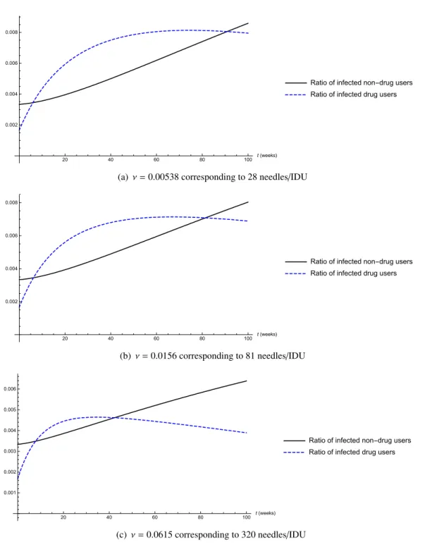
Figure 4 shows the number of infected non-drug users, resp. IDUs for different rates of sterile needle distribution. The first figure shows the situation after the reduction of the needle exchange program, when 28 needles/IDU were distributed yearly. In this case, the reproduction number takes the value R0 = 1.294. In the second figure, one can see the situation before the reduction of the program, when 81 needles/IDU were provided yearly. The basic reproduction number significantly decreases, though it is still above 1, taking the valueR0 = 1.11. The third figure shows the case of 320 needles
distributed/IDU. In this case, the reproduction number decreases below 1, with R0 = 0.9035. Hence, these simulations suggest that a significant number of new infections could have been spared with keeping the earlier level of sterile needle distribution, moreover, a further increase of the number of new needles could have even driven the reproduction number below 1.
20 40 60 80 100 t(weeks)
0.002 0.004 0.006 0.008
Ratio of infected non-drug users Ratio of infected drug users
(a)ν=0.00538 corresponding to 28 needles/IDU
20 40 60 80 100 t(weeks)
0.002 0.004 0.006 0.008
Ratio of infected non-drug users Ratio of infected drug users
(b)ν=0.0156 corresponding to 81 needles/IDU
20 40 60 80 100 t(weeks)
0.001 0.002 0.003 0.004 0.005 0.006
Ratio of infected non-drug users Ratio of infected drug users
(c) ν=0.0615 corresponding to 320 needles/IDU
Figure 4. The ratio of infected non-drug users and IDUs for different needle distribution rates (time shown in weeks).
6.2. Fitting of the model with time-dependent needle distribution parameter—a case study for Hungary
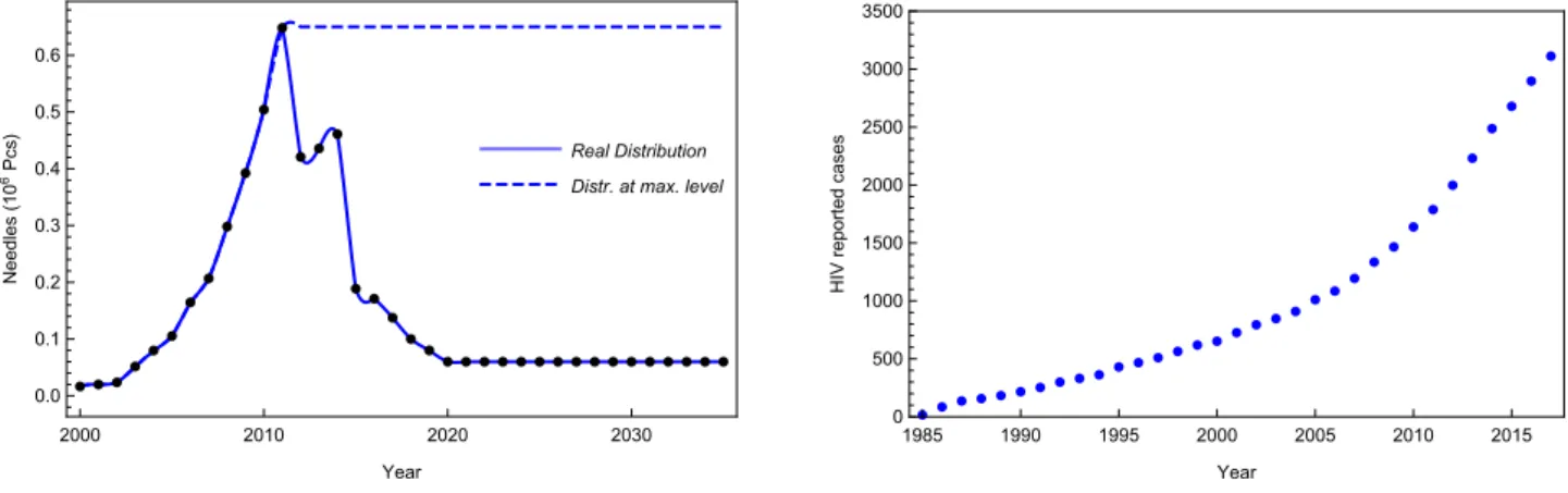
According to the world-wide situation, the number of HIV infected individuals and intravenous drug users is increasing. The budget of the needle exchange program has been reduced recently in Hungary.
The number of reported cases and distributed needles can be seen in Figure 5. Needle distribution is extrapolated from 2018 to 2035 at the current low level as well as at the highest level for further study.
2000 2010 2020 2030
0.0 0.1 0.2 0.3 0.4 0.5 0.6
Year Needles(106Pcs)
Real Distribution Distr. at max. level
1985 1990 1995 2000 2005 2010 2015
0 500 1000 1500 2000 2500 3000 3500
Year
HIVreportedcases
Figure 5. Needle distribution and HIV spreading in Hungary.
Our model given in system (2.1) cannot be directly applied to this case, since the needle distribution is changing from year to year. Hence, instead of the constant needle exchange rate ν, we introduce the rate functionν(t) interpolated to the given data. This non-autonomous system is fitted to the HIV cases from 2000 to 2017. Because of the high number of parameters, many of them are taken from the literature (see above) or fixed by some assumptions. In addition, by our experience, some kind of underreporting has to be taken into account, as well.
In the study we made the following assumptions. HIV infected and intravenous drug user populations are quite closed, we assume that the exposed population is about 100000 (estimated:
population between 11 and 65 years, living in cities, having exposed life style). The death rate in Hungary isλ≈0.01, we keep it, due to the higher rate in this population.
Concerning the epidemiology and further parameters: we have the following assumptions: λ = 0.01, a = 0.06, g = 0.0225, α = 0.15, β = 0.06. Due to the uncertainties, parameters concerning the needle infections/disinfectionsθ, ωare used in the fitting. The model including the underreporting ratioqis simple: Model(q, θ, ω)(t)=q(I(t)+ID(t)), whereI(t), ID(t) are solutions of (2.1).
Note that the fitting is very sensitive to the initial values. They are taken from and estimated by the available data at 2000 [24, 25, 30], and corrected by the underreporting ratioq:I(0)=0.006/q, ID(0)= 0.0004/q, SD(0)= 0.0026,S(0)=1−I(0)−ID(0)−SD(0).
Taking into account that the number of collected used needles is about 60% of new ones [30] and that the number of HIV infected and intravenous drug users are increasing, we assume that altogether 106needles are in use, and only 15% of needles were infected in 2000, hence: SN(0)= 0.85; IN(0) = 0.15. For numerical studies, we useWolfram Mathematica 11.3commandsParametricNDSolveand NonlinearModelFit. The commandParametricNDSolvenumerically solves differential equations
with undefined parameters by creating aParametricFunction object, and enables to work with the solutions as if they were given symbolically. Fitting was performed by the sophisticated and well-tested commandNonlinearModelFit, which can be applied to implicitly defined models such as numerical solutions of differential equations provided byParametricNDSolve, and it can measure the goodness of fitting. Default options andConfidenceLevel→0.95 were used.
The result of the fitting is presented in Table 2. Although by changing our assumptions the result would certainly be different, the main problems are well visible now. Underreporting is high, due to the nature of HIV, the ratio of hidden cases is significant, and it fits the general opinion among epidemiologists. The sterilization rate of needles (θ) is low as expected, and the high rate of infection of needles (ω) is in correspondence with this.
Table 2. Result of the fitting to HIV data in Hungary; 90% confidence level.
Estimate Standard Error Confidence Interval
q 0.373 0.063 [0.239,0.5063]
θ 0.362 0.0315 [0.295,0.429]
ω 1.193 0.105 [0.970,1.416]
Finally, Figures 6, 7 and 8 present graphically the fitting and forecast. In Figure 6 continuous red line shows the model I(t)+ ID(t) fitted to the corrected data (blue dotted line) using the real needle distribution (see Figure 5). The dashed red line shows the trend of the model (using the same parameters) if the needle distribution were at the highest level, approximately 650000 needles/year.
Figure 7 shows the accumulated number of infected non-drug users (I) and infected drug users (ID).
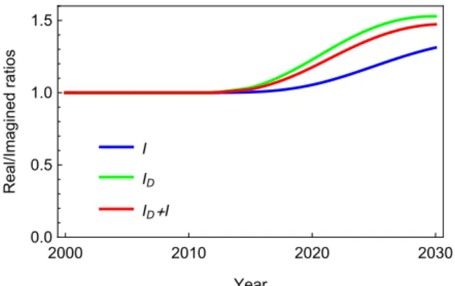
Figure 8 shows the ratio of the two values of the compartmentsI, ID, resp. I+ID obtained in the real and in the imagined model. The figures illustrate very well that the decrease of needle exchange dramatically increase the ratio of drug user infected persons Id, hence it is responsible for the high value of I as well. The difference in 2030 is more than significant between these two estimates, even if these results are quite hypothetic under the assumptions of our models.
2000 2010 2020 2030
0.0 0.1 0.2 0.3 0.4
Year
ID+I(105persons) Real model
Imagined model Corrected Data Original Data
Figure 6. HIV spreading in Hungary: data, and fitted models.
2000 2010 2020 2030 0.0
0.1 0.2 0.3 0.4
Year IandID+I(105persons)
Real model
I ID+I
2000 2010 2020 2030
0.0 0.1 0.2 0.3 0.4
Year IandID+I(105persons)
Imagined model
I ID+I
Figure 7. Real and imagined models: compartmentsIandIDaccumulated.
2000 2010 2020 2030
0.0 0.5 1.0 1.5
Year
Real/Imaginedratios
I ID ID+I
Figure 8. Ratio of values of the compartments I, ID, resp. I + ID in the real and in the imagined model.
7. Discussion
In this paper, we have established a new model to study the spread of a sexually transmitted disease through sexual transmission and the use of contaminated needles among intravenous drug users. Beyond determining the dynamics of the model, our aim was to study in what extent the recent reduction of needle exchange programs in several countries indirectly affects non-drug users via sexual contacts with infected intravenous drug users. We first determined the basic reproduction numberR0 of the system and showed that forR0 < 1, the unique disease-free equilibrium is globally asymptotically stable. In the caseR0 > 1, the disease was shown to persist in the population. Using numerical simulations, we showed that the reduction of the needle exchange program can highly contribute to the spread of diseases not only among drug users, but also among those who do not use drugs, while an increased program can contribute to the eradication of these diseases. Based on real world data from Hungary, we gave a forecast for the number of HIV infections for the next decade.
We also compared the number of HIV infections with the current tendency of the needle exchange
program and a situation where the original high level of distribution is maintained. This simulation suggests that a significant number of new infections could be avoided with the help of the needle exchange program. Of course, the model has certain limitations. For example, for a more realistic result, one should consider several subgroups corresponding to different tendencies of drug use, needle sharing and risky sexual behaviour. The homogeneous mixing assumption may lead to an overestimation of the impact of needle exchange programs on HIV prevalence for non-drug users.
HIV being a sexually transmitted disease, a more realistic model should differentiate sexes and subgroups with different transmission probabilities. These generalizations of our model are the topic of a future work.
Acknowledgements
This research was supported by the Ministry of Human Capacities, Hungary grant 20391-3/2018/FEKUSTRAT. A. D´enes was supported by the J´anos Bolyai Research Scholarship of the Hungarian Academy of Sciences, by the project no. 125119, implemented with the support provided from the National Research, Development and Innovation Fund of Hungary, financed under the SNN 17 funding scheme and by the project no. 128363, implemented with the support provided from the National Research, Development and Innovation Fund of Hungary, financed under the PD 18 funding scheme. J. Karsai was supported by the project no. 125628, implemented with the support provided from the National Research, Development and Innovation Fund of Hungary, financed under the KH 17 funding scheme and by the EU-funded Hungarian grant EFOP-3.6.2-16-2017-00015. L. Sz´ekely was supported by the EU-funded Hungarian grant EFOP-3.6.1-16-2016-00008. The authors are grateful to Dr. Gergely R¨ost for his useful suggestions.
Conflict of interest
The authors declare there is no conflict of interest.
References
1. W. Atkinson, J. Hamborsky, L. McIntyre, et al., Hepatitis B, in: J. E. Bennett, R. Dolin, M.
J. Blaser (Eds.), Epidemiology and prevention of vaccine-preventable diseases (The Pink Book), pp. 211–234. Public Health Foundation, Washington DC, 2009.
2. N. Scherbaum, B. T. Baune, R. Mikolajczyk, et al., Prevalence and risk factors of syphilis infection among drug addicts, BMC Infect. Dis.5(2005), 6.
3. Centers for Disease Control and Prevention, HIV Basics, available at: https://www.cdc.gov/
hiv/basics/index.html.
4. N. Loimer, R. Schmid and A. Springer (eds), Drug addiction and AIDS, Springer, 1991.
5. A. J. Saxon, D. A. Calsyn, S. Whittaker, et al., Sexual behaviors of intravenous drug users in treatment, J. Acquir. Immune Defic. Syndr.,4(1991), 938–944.
6. Y. Yao, K. Smith, J. Chu, et al., Sexual behavior and risks for HIV infection and transmission among male injecting drug users in Yunnan, China, Int. J. Infect. Dis.,13(2009), 154-–161.
7. D. Hedrich, E. Kalamara, O. Sfetcu, et al., Human immunodeficiency virus among people who inject drugs: Is risk increasing in Europe?, Euro Surveill.,48(2013).
8. S. Mushayabasa and C. P. Bhunu, Hepatitis C virus and intravenous drug misuse: a modeling approach, Int. J. Biomath.,7(2014), 22 pp.
9. C. P. Bhunu and S. Mushayabasa, Assessing the effects of intravenous drug use on Hepatitis C transmission dynamics, J. Biol. Syst.,19(2011), 447–460.
10. J. Gani, Needle sharing infections among heterogeneous IVDUS, Monatsh. Math., 135 (2002), 25–36.
11. Y. Ji, S. Kumar and S. Sethi, Needle exchange for controlling HIV spread under endogenous infectivity, INFOR Inf. Syst. Oper. Res.,55(2017), 93–117.
12. E. H. Kaplan and R. Heimer, HIV prevalence among intravenous drug users: model-based estimates from New Haven’s legal needle exchange, J. Acquir. Immune Defic. Syndr., (1992), 163–169.
13. E. H. Kaplan and E. O’Keefe, Let the needles do the talking! Evaluating the New Haven needle exchange, Interfaces,23(1993), 7–26.
14. E. H. Kaplan and R. Heimer, A model based estimate of HIV infectivity via needle sharing, J.
Acquir. Immune Defic. Syndr.,5(1992), 1116–1118.
15. D. Greenhalgh and W. Al-Fwzan, An improved optimistic three stage model for the spread of HIV amongst injecting intravenous drug users, Discrete Contin. Dyn. Syst., Supplement 2009, 286–299.
16. D. Greenhalgh and F. Lewis, The general mixing of addicts and needles in a variable-infectivity needle-sharing environment, J. Math. Biol.,44(2002), 561–598.
17. F. Lewis and D. Greenhalgh, Three stage AIDS incubation period: a worst case scenario using addict–needle interaction assumptions, Math. Biosci.,169(2001), 53–87.
18. E. H. Kaplan, Needles that kill: modeling human immunodeficiency virus transmission via shared drug injection equipment in shooting galleries, Rev. Infect. Dis.,11(1989), 289–298.
19. R. F. Baggaley, M-C. Boily, R. G. White, et al., Risk of HIV-1 transmission for parental exposure and blood transfusion: a systematic review and meta-analysis, AIDS,20(2006), 805–812.
20. Centers for Disease Control and Prevention, HIV in the United States, 2017, available from:
https://www.cdc.gov/hiv/statistics/overview/ataglance.html.
21. Centers for Disease Control and Prevention, HIV risk behaviors. Estimated per-act probability of acquiring HIV from an infected source, by exposure act, available from: https://www.cdc.
gov/hiv/risk/estimates/riskbehaviors.html
22. O. Diekmann, J. A. P. Heesterbeek and M. G. Roberts, The construction of next-generation matrices for compartmental epidemic models, J. R. Soc. Interface,7(2010), 873–885.
23. L. Farina and S. Rinaldi,Positive linear systems. Theory and applications, John Wiley AND Sons, 2000.
24. Hungarian AIDS foundation, HIV/AIDS statistics for Hungary (in Hungarian), available from:
http://www.aidsinfo.hu/statisztika_magyar_t.
25. Hungarian National Focal Point, Facts and figures about the needle exchange programs, available from: http://drogfokuszpont.hu/szakteruleteink/artalomcsokkentes/
artalomcsokkentes-tenyek-es-szamok/?lang=en
26. J. P. LaSalle, Stability by Liapunov’s direct method, with applications, Mathematics in Science and Engineering, Academic Press, New York, 1961.
27. Z. Shuai and P. van den Driessche, Global stability of infectious disease models using Lyapunov functions, SIAM J. Appl. Math.,73(2013), 1513–1532.
28. H. Smith, An introduction to delay differential equations with applications to the life sciences, Springer, New York, 2011.
29. H. L. Smith and H. R. Thieme, Dynamical systems and population persistence, Graduate Studies in Mathematics, Vol. 118, AMS, Providence, 2011.
30. Hungarian National Focal Point, 2018 National Report to the EMCDDA by the Reitox National Focal Point, available from: http://drogfokuszpont.hu/wp-content/uploads/
HU_EMCDDA_jelentes_HUNGARY_2018_EN.pdf c
2019 the Author(s), licensee AIMS Press. This is an open access article distributed under the terms of the Creative Commons Attribution License (http://creativecommons.org/licenses/by/4.0)