Including Ectoparasites, Rodents and Humans
A. Dénes and G. Röst
1 Introduction
Ectoparasites are parasites that live on or in the skin but not within the body. These parasites, e.g. lice, fleas, mites have long been known as vectors of several infectious diseases including epidemic typhus and plague. It is also commonly known that in several cases, ectoparasites are transmitted to humans from animals, most often by rodents. A well-known example for this is plague, caused by the bacterium Yersinia pestis: the fleas transmitting this disease were transmitted to humans by rats [5]. Other notable examples are Omsk haemorrhagic fever, caused by a Flavivirus transmitted by ticks on water voles and muskrats [4]; rickettsialpox, caused by the bacteriaRickettsia akaritransmitted by mites on mice [6]; murine typhus, caused by the bacteriaRickettsia typhi, transmitted by fleas, usually on rats [9]; scrub typhus caused by the parasiteOrientia tsutsugamushi, transmitted by trombiculid mites, carried by mice. The latter disease is estimated to cause more than a million cases annually in Asia with more than a billion people being at risk, which makes scrub typhus the most medically important rickettsial disease [10] (Figs.1and2).
In this work, we consider an infectious disease caused by a pathogen spread by ectoparasites which are harboured by rodents. We assume that ectoparasites spread by the rodents might be infectious or non-infectious. A given rodent or human can be infested only by one type (either infectious or non-infectious) of the ectoparasite. A human can be infested (and hence possibly infected) through adequate contact with an infested (infected) rodent or another human. We assume that the ectoparasites are not transmitted back from humans to the rodents. Due to infestation and/or treatment, infested and infected humans may become susceptible again.
A. Dénes () · G. Röst
Bolyai Institute, University of Szeged, Szeged, Hungary e-mail:denesa@math.u-szeged.hu
© Springer International Publishing AG, part of Springer Nature 2018 R. P. Mondaini (ed.),Trends in Biomathematics: Modeling, Optimization and Computational Problems,https://doi.org/10.1007/978-3-319-91092-5_5
59
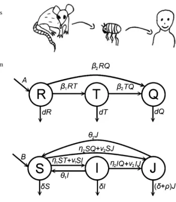
Fig. 1 The pathogen can jump from rodents to humans via ectoparasites. Figure:
courtesy of Júlia Röst
Fig. 2 Transmission diagram representing transitions between the rodent and the human compartments
The structure of the paper is as follows. In Sect.2, we establish a compartmental model describing the spread of the infestation and the disease. In Sect.3, we study the subsystem formed by the equations for the rodent compartments, while, using the results of Sect.3, we study the human subsystem in Sect.4.
2 The Model
We denote by R(t) the compartment of susceptible rodents, T (t)stands for the rodents infested by non-infectious parasites, while Q(t) denotes the number of rodents infested by infectious parasites. Similarly, we have three compartments for the humans: S(t)denotes susceptibles, I (t) those infested by non-infectious parasites, andJ (t)those infested by infectious parasites.Aanddstand for the birth, resp. death rates of rodents. The notationβ1stands for the transmission rate between the compartmentsRandT, whileβ2is the transmission rate betweenRandQ, resp.
T andQ.Bandδstand for natural birth and death rates for humans, andρdenotes disease-induced death rate for the infected human compartmentJ. The parameter ν1denotes transmission rate between the compartmentsSandI, whileν2denotes transmission rate fromJtoSandJ toI. The parameterη1denotes the transmission rate from rodents infested by non-infectious parasites to susceptible humans, while
η2is the transmission rate from rodents infested by infectious parasites to humans.
We denote byθ1, resp.θ2the disinfestation, resp. recovery rate from compartments I, resp.J.
Using the above notations, our equations take the following form:
R(t)=A−β1R(t)T (t)−β2R(t)Q(t)−dR(t), T(t)=β1R(t)T (t)−β2T (t)Q(t)−dT (t), Q(t)=β2R(t)Q(t)+β2T (t)Q(t)−dQ(t),
S(t)=B−η1S(t)T (t)−η2S(t)Q(t)−ν1S(t)I (t)−ν2S(t)J (t)
−δS(t)+θ1I (t)+θ2J (t), I(t)=η1S(t)T (t)+ν1S(t)I (t)
−η2I (t)Q(t)−ν2I (t)J (t)−δI (t)−θ1I (t), J(t)=η2S(t)Q(t)+η2I (t)Q(t)+ν2S(t)J (t)+ν2I (t)J (t)
−δJ (t)−ρJ (t)−θ2J (t),
(1)
with positive initial conditionsR(0), T (0), Q(0), S(0), I (0), J (0)≥0. The phase space
R6+= {(R, T , Q, S, I, J )∈R6:R, T , Q, S, I, J ≥0} is clearly invariant to system (1).
3 The Rodent Subsystem 3.1 Equilibria, Local Stability
The first three equations of (1) can be decoupled from the remaining ones. The subsystem for the spread among rodents, given by
R(t)=A−β1R(t)T (t)−β2R(t)Q(t)−dR(t), T(t)=β1R(t)T (t)−β2T (t)Q(t)−dT (t), Q(t)=β2R(t)Q(t)+β2T (t)Q(t)−dQ(t)
(2)
has a similar structure as the model given by Dénes and Röst [1,2], though, in the present case, birth and death rates are not equal in contrast to the cited papers.
To calculate the equilibria of the full system, we start by calculating those of the rodent subsystem (2), which are easily obtained by solving the algebraic system of equations
0=A−β1RT −β2RQ−dR, 0=β1RT −β2T Q−dT , 0=β2RQ+β2T Q−dQ, resulting in the four possible equilibria
ER=A
d,0,0
, ET =
βd1,Ad −βd1,0 EQ=
βd2,0,Ad −βd2
, ETQ=
Aβ2
dβ1,βd2 −Aβdβ12,Ad −βd2 .
(3)
By introducing a single infested/infected individual into one of the equilibriaER, ET andEQ, we obtain three different reproduction numbers. If we introduce a rodent infested by the non-infectious parasites into the disease- and infestation-free equilibrium, we obtain the reproduction numberr1= Aβd21.
Introducing a rodent infested by the infectious parasites into the equilibriumER, we obtain the reproduction numberr2= Aβd22.
If we introduce a rodent infested by the infectious parasites into the equilibrium ET, we obtain again the same reproduction numberr2. Finally, let us introduce a rodent infested by the non-infectious parasites into the equilibriumEQ. In this case, the expected sojourn time of an individual infected with the first strain in theT- compartment is(β2Q∗+d)−1, and the number of new infections generated by this individual isβ1R∗, whereR∗andQ∗stand for the first, resp. third coordinates of the equilibriumEQ. This way we obtain the reproduction numberr3=β1d2
β22A. It is obvious that the equilibriumERalways exists,ET exists if and only ifr1>
1,EQexists if and only ifr2>1, whileET Qexists if and only ifr2>1 andr3>1.
The following proposition on the local stability of the four equilibria can easily be checked, see [3].
Proposition 3.1 The disease-free equilibriumER is locally asymptotically stable if r1 < 1 and r2 < 1 and unstable if r1 > 1 orr2 > 1. The equilibrium ET
is locally asymptotically stable if r1 > 1 and r2 < 1. The equilibrium EQ is locally asymptotically stable ifr2>1andr3<1. The equilibriumET Qis locally asymptotically stable ifr2>1andr3>1.
3.2 Persistence
Before we can state our results on the persistence of the three compartments, we will need some notions and theorems from [8].
Definition 3.1 LetXbe a nonempty set andρ:X → R+. A semiflow:R+× X → X is called uniformly weaklyρ-persistent, if there exists someε > 0 such that lim supt→∞ρ((t, x)) > εfor allx ∈ X, ρ(x) > 0.is calleduniformly
(strongly)ρ-persistentif there exists someε >0 such that lim inft→∞ρ((t, x)) >
εfor allx ∈X, ρ(x) >0. A setM⊆Xis calledweaklyρ-repellingif there is no x∈Xsuch thatρ(x) >0 and(t, x)→Mast → ∞.
System (2) generates a continuous flow on the phase space
X:=
(R, T , Q)∈R3+ .
Theorem 3.1 R(t)is always uniformly persistent.T (t)is uniformly persistent if r1>1andr2 <1as well as ifr2>1andr3>1.Q(t)is uniformly persistent if r2>1.
Proof To show uniform persistence of the susceptible compartment, we will use the method of fluctuation (see, e.g., [7, Lemma A.1]). We denote byR∞the limit inferior ofR(t), whileT∞ andQ∞denote the limit superior ofT (t), resp.Q(t) ast → ∞. Using the fluctuation lemma we know that there exists a time sequence tk → ∞such thatR(tk)→R∞andR(tk)→0 ask→ ∞. If we apply this to the equation forR(t), we obtain
R(tk)+β1R(tk)T (tk)+β2R(tk)Q(tk)=A.
It is easy to see that for the total rodent population we haveR(t)+T (t)+Q(t)→ Ad, thus, 0 ≤ T∞ ≤ Ad and 0 ≤ Q∞ ≤ Ad. Using this and lettingk → ∞we get R∞≥ β1+βd 2.
To show persistence of the infested compartments, we need some theory from [8]. We use the notationx = (R, T , Q) ∈ X for the state of the system and the usual notationω(x)for theω-limit set of a pointxdefined as
ω(x):= {y ∈X: ∃{tn}n≥1s. t.tn→ ∞and(tn, x)→yasn→ ∞}.
We first show the persistence ofT (t). Letρ(x)=T. Let us consider the invariant extinction space ofT, defined as XT := {x ∈ X : ρ(x) = 0}. We follow [8, Chapter 8] and examine the setx∈XT := ∪x∈XTω(x). Applying the Bendixson–
Dulac criterion with Dulac function 1/Qand the Poincaré–Bendixson theorem, we obtain that all solutions in the extinction spaceXT tend to an equilibrium.
Let us first consider the caser1>1 andr2≤1. Clearly, in this case= {ER}.
As a first step, we prove weakρ-persistence. In order to apply [8, Theorem 8.17], we letM1= {ER}. Thenis a subset ofM1, which is isolated, compact, invariant and acylic. We have to show thatM1is weaklyρ-repelling, from which we obtain persistence.
Let us suppose that this does not hold, i.e. there exists a solution such that limt→∞(R(t), T (t), Q(t)) = (Ad,0,0) andT (t) > 0. Then for any ε > 0, for sufficiently larget, we haveR(t) > Ad −εandQ(t) < ε. For sucht, we can give the following estimation forT(t):
T(t)=T (t)(β1R(t)−β2Q(t)−d) > T (t)
β1Ad −β1ε−β2ε−d , which is positive ifεis sufficiently small as Aβd1 > d follows fromr1 > 1. This contradictsT (t)→0.
In the second case, whenr2 >1 andr3 > 1, alsoEQexists, so we have = {ER, EQ}. Now we letM1 = {ER}andM2 = {EQ}. Clearly,⊂M1∪M2and {M1, M2}is acyclic andM1andM2are invariant, compact and isolated. We have to show thatM1andM2are weaklyρ-repelling.
Suppose first thatM1is not weaklyρ-repelling. Then there exists a solution such that limt→∞(R(t), T (t), Q(t))=(Ad,0,0)andT (t) >0. Again, for anyε >0, for sufficiently larget, we haveR(t) >Ad andQ(t) < εand for sucht, we can give the following estimation forT(t):
T(t)=T (t)(β1R(t)−β2Q(t)−d) > T (t)
β2Ad −β1ε−β2ε−d , where we used that β1 > β2, which follows from r2r3 > 1. This expression is positive forεsmall enough, which contradictsT (t)→0.
Now let us suppose thatM2is not weaklyρ-repelling. Then there exists a solution such that limt→∞(R(t), T (t), Q(t))=d
β2,0,Ad −βd2
. Then, for anyε >0, iftis large enough, thenR(t) > βd2 −εandQ(t) < Ad − βd2 +εand for sucht we can give the following estimation forT(t):
T(t)=T (t)(β1R(t)−β2Q(t)−d)
> T (t) dβ1
β2 −β1ε−β2
A
d −βd2 +ε −d
=T (t) dβ1
β2 −Aβd2 −(β1+β2)ε
,
which is positive forεsmall enough asr3>1. This contradictsT (t)→0.
Let us now turn to the persistence ofQ(t)in the caser2>1. We setρ(x)=Q. We have the equilibriumERifr1≤1 and the two equilibriaERandET ifr1>1.
Similarly to the case ofT (t), we define the extinction space ofQasXQ := {x ∈ X:ρ(x)=0} = {(R, T ,0)∈R3+}. In this case we have= ∪x∈XQω(x)= {ER} ifr1≤1 and= ∪x∈XQω(x)= {ER, ET}ifr1>1. We defineM1= {ER}and M2= {ET}. Just like in the proof of the persistence ofT (t),is invariant, andM1 andM2are isolated and acyclic.
To show thatM1is weaklyρ-repelling, we can proceed in an analogous way as in the case ofT (t).
In the caser1>1, we have to show thatM2is weaklyρ-repelling. Suppose this does not hold. Then there exists a solution such that limt→∞(R(t), T (t), Q(t)) = (βd1,Ad −βd1,0)andQ(t) > 0. Then, for anyε > 0, ift is sufficiently large, then R(t) > βd1 −εandT (t) > Ad −βd1 −εand for sucht we can give the following estimation forQ(t):
Q(t)=Q(t)(β2R(t)+β2T (t)−d)
> Q(t)
β2 d
β1 −ε +β2
A
d −βd1 −ε −d
=Q(t) Aβ2
d −d−2β2ε
,
which is positive ifεis small enough, asr2>1, which contradictsQ(t)→0.
We have shown uniform weak persistence in all cases; to show uniform (strong) persistence, we apply Theorem 4.5 from [8]. Our flow is clearly continuous, the subspacesXT, XQ, X\XT andX\XQare invariant. The existence of a compact attractor is also clear, as all solutions enter a compact region after some time. This means that all conditions of [8, Theorem 4.5] hold and thus we obtain uniform strong
persistence.
3.3 Global Stability
Theorem 3.2
(1) EquilibriumERis globally asymptotically stable ifr1<1andr2<1.
(2) EquilibriumET is globally asymptotically stable on X\XT if r1 > 1 and r2<1.ERis globally asymptotically stable onXT.
(3) EquilibriumEQ is globally asymptotically stable onX\XQif r2 > 1 and r3<1.ERis globally asymptotically stable onXQifr1<1andET is globally asymptotically stable onXQifr1>1.
(4) EquilibriumETQis globally asymptotically stable onX\(XT ∪XQ)ifr2>1 and r3 > 1.ET is globally asymptotically stable onXQ andEQis globally asymptotically stable onXT.
Proof First we note that the rodent subsystem (2) can be reduced to two dimensions by introducing the notationF (t):=R(t)+T (t). We obtain the system
F(t)=A−β2F (t)Q(t)−dF (t),
Q(t)=β2F (t)Q(t)−dQ(t). (4)
This system has two equilibria,A
d,0 andd
β2,Ad − βd2
, with the latter one only existing ifr2>1. We use the Dulac function 1/Qto show that there is no periodic solution of (4):
∂
∂F
A−β2F Q−dF
Q + ∂
∂Q
β2F Q−dQ
Q = −β2− d
Q<0.
Thus, applying the Bendixson–Dulac criterion, we obtain that there is no periodic solution of (4), and by the Poincaré–Bendixson theorem we get that all solutions tend to an equilibrium.
In the first two cases, whenr2<1, only the first equilibrium exists. Thus, in this caseQ(t)→0 andF (t)→ Ad ast → ∞, and therefore, the second equation of (2) takes the following form on the limit set:
T(t)=β1
A
d −T (t)
T (t)−dT (t)=γ T (t)−β1T2(t) withγ =Aβ1
d −d .
The solution started fromT (t)=0 is the constant solutionT (t)≡0, while the nontrivial solutions take the form
Ceγ t
1+βγ1Ceγ t (5)
forC ∈R+. Clearly, forr1<1 (which is equivalent toγ ≤ 0), the solutions tend to zero on the limit set, therefore, for all solutions,T (t)→0 ast→ ∞.
Ifr1 >0 (i.e.γ > 0), we have limt→∞T (t)= Ad −βd
1 on the limit set; using the persistence ofT (t)we obtain that for all solutions,T (t)→ Ad −βd1 ast→ ∞.
In the case r2 > 1, also the second equilibrium exists. However, we know from the previous subsection that forr2 > 1, the compartmentQ(t)is uniformly persistent, so no solution with positive initial value inQ(t) can tend to the first equilibrium. Thus, the limit of all such solutions is the second equilibrium and Q(t) → (Ad − βd2)as t → ∞. We can proceed in a similar way as in the case r2<1: on the limit set, we can transform the second equation of (2) to
T(t)=β1
d
β2 −T (t)
T (t)−β2
A d −βd2
T (t)−dT (t)
=γ T (t)−β1T2(t) withγ =dβ1
β2 −Aβd2
. Similarly as above, we can see that the solution started from T (t)=0 is the constant solutionT (t)≡0, while the nontrivial solutions take the form (5). In the caser3<1 (which is equivalent toγ ≤0), the solutions tend to 0, while ifr3>1 (which is equivalent toγ >0), we have limt→∞T (t)=βd2 −Aβdβ12,
and this is what we wanted to show.
Remark 3.1 We note that changing global asymptotic stability to attractivity, the results of Theorem3.2also hold when the given reproduction numbers are equal to 1, instead of being smaller than 1.
4 The Human Subsystem
Let us now turn to the human subsystem of (1) consisting of the last three equations.
In the sequel, we assume that the rodent subsystem is in a steady state, and substitute any of the equilibria of the rodent subsystem into these equations to obtain the system
S(t)=B−η1T∗S(t)−η2Q∗S(t)−ν1S(t)I (t)−ν2S(t)J (t)
−δS(t)+θ1I (t)+θ2J (t), I(t)=η1T∗S(t)+ν1S(t)I (t)
−η2Q∗I (t)−ν2J (t)I (t)−δI (t)−θ1I (t), J(t)=η2Q∗S(t)+η2Q∗I (t)+ν2S(t)J (t)+ν2I (t)J (t)
−δJ (t)−ρJ (t)−θ2J (t),
(6)
where T∗ and Q∗ are the second, resp. third coordinates in any of the four equilibria (3).
To find all possible equilibria of (6), first we introduce the notation G(t) :=
S(t)+I (t)to obtain the system
G(t)=B−η2Q∗G(t)−ν2G(t)J (t)−δG(t)+θ2J (t),
J(t)=η2Q∗G(t)+ν2G(t)J (t)−δJ (t)−ρJ (t)−θ2J (t). (7) We will apply the Bendixson–Dulac criterion with Dulac function 1/J and the Poincaré–Bendixson theorem to obtain that in this case, all solutions of system (7) tend to one of the equilibria. Indeed, we have
∂
∂G
B−η2Q∗G−ν2GJ −δG+θ2J J
+ ∂
∂J
η2Q∗G+ν2GJ−δJ−ρJ−θ2J J
= −η2Q∗
J −ν2− δ J −η2G
J2 <0, from which we obtain the assertion above.
This equation may have two equilibria:
D+Bν2−√
(D−Bν2)2+4Bη2Q∗ν2(δ+ρ)
2δν2 ,−D+Bν2+
√(D−Bν2)2+4Bη2Q∗ν2(δ+ρ) 2(δ+ρ)ν2
and
D+Bν2+√
(D−Bν2)2+4Bη2Q∗ν2(δ+ρ)
2δν2 ,−D+Bν2−
√(D−Bν2)2+4Bη2Q∗ν2(δ+ρ) 2(δ+ρ)ν2
denoted byE1andE2, respectively, withD=δ2+Q∗η2ρ+δ(Q∗η2+θ2+ρ). The first coordinate ofE1is always positive, since this coordinate may be rewritten as
D+Bν2−
(D+Bν2)2−4Bδν2(δ+θ2+ρ)
2δν2 .
It can easily be seen that the first coordinate ofE2is always positive.
Let us first consider the caseQ∗ >0, (i.e. when the rodent subsystem tends to the equilibriumEQorETQ, which is equivalent tor2>1). In this case, the second coordinate ofE1 is always positive, while second coordinate ofE2is negative if Q∗ > 0. Hence, in the caseQ∗ >0, there is only one equilibrium and using the Poincaré–Bendixson theorem, we obtain that all solutions tend toE1.
In the caser2≤1, i.e. whenQ∗=0, the system takes the simpler form G(t)=B−ν2G(t)J (t)−δG(t)+θ2J (t),
J(t)=ν2G(t)J (t)−δJ (t)−ρJ (t)−θ2J (t). (8) This system has the two equilibria
e1:=
B δ,0
and e2:=
δ+θ2+ρ
ν2 ,Bν2−δ(δ+θ2+ρ) ν2(δ+ρ)
. Now, it is easy to see that the first of these equilibria always exists, while the second one only exists if
RJ0 := Bν2
δ(δ+θ2+ρ) >1.
Just as above, we obtain that all solutions of (8) tend to one of these equilibria. In the caseRJ0 ≤ 1,this equilibrium is clearlye1. Using similar methods as for the rodent subsystem, we will show thatJ (t) is always uniformly strongly persistent ifRJ0 >1. To show this, we chooseρ(x)=J. Consider the extinction spaceXJ
defined asXJ := {x ∈R2+ : ρ(x)=0}; now=M1 :=e1, which is obviously invariant, isolated and acyclic. Let us suppose thatM1is not weaklyρ-repelling, i.e.
there is a solution which tends toe1such thatJ (t) >0. Then, given anyε >0, for tsufficiently large, we can give the following estimate forJ(t):
J(t)=ν2G(t)J (t)−δJ (t)−ρJ (t)−θ2J (t)
> J (t) ν2B
δ −ν2ε−δ−ρ−θ2
,
which is positive asRJ0 >1. Hence, in the caseRJ0 >1, all solutions of (8) started with positive initial valueJ (0)tend to the equilibriume2.
We have now finished the analysis of (7) and showed that in each case, depending on the reproduction numbersr2 andRJ0, all solutions of this equation tend to an equilibrium. Let us denote by J∗ the second coordinate of this equilibrium and substitute this value into the first two equations of (6) to obtain
S(t)=B−η1T∗S(t)−η2Q∗S(t)−ν1S(t)I (t)−ν2J∗S(t)
−δS(t)+θ1I (t)+θ2J∗,
I(t)=η1T∗S(t)+ν1S(t)I (t)−η2Q∗I (t)
−ν2J∗I (t)−δI (t)−θ1I (t).
(9)
This equation has a similar structure as (7). The two possible equilibria of system (9) are
ν1(B+θ2J∗)+P−√
(ν1(B+θ2J∗)−P )2+H
2ν1K ,ν1(B+θ2J∗)−P+
√(ν1(B+θ2J∗)−P )2+H 2ν1K
and
ν1(B+θ2J∗)+P+√
(ν1(B+θ2J∗)−P )2+H
2ν1K ,ν1(B+θ2J∗)−P−
√(ν1(B+θ2J∗)−P )2+H 2ν1K
denoted byE1 andE2, respectively, where the notationsK,P andH are defined asK =(δ+η2Q∗+ν2J∗),P =K(δ+θ1+η1T∗+η2Q∗+ν2J∗)andH = 4η1ν1T∗(B+θ2J∗)K. Again, we can apply the Bendixson–Dulac criterion, in this case with the Dulac function 1/I, to show that all solutions tend to an equilibrium:
∂
∂S
B−η1T∗S−η2Q∗S−ν1SI −ν2J∗S−δS+θ1I+θ2J∗ I
+ ∂
∂I
η1T∗S+ν1SI−η2Q∗I −ν2J∗I−δI−θ1I I
= −η1T∗
I −η2Q∗
I −ν1−ν2J∗ I −δ
I −η1T∗S I2 , which is negative for allI, S >0.
Similarly as in the case of the equilibria of system (7), it is easy to see that the first coordinates ofE1andE2are always positive, while the second coordinate of E2 is negative ifT∗ > 0 (i.e. whenr1 > 1 and r2 < 1, meaning thatET is globally asymptotically stable orr2>1 andr3 >1 meaning thatETQis globally asymptotically stable). Hence, in this case there is only one equilibrium, and by the Poincaré–Bendixson theorem, all solutions tend to this equilibrium.
From the above, we obtain that ifT∗ > 0 andQ∗ > 0, i.e. whenr2 >1 and r3>1, then all solutions tend to the equilibrium(E11,E12, E21), where upper indexi denotes theith coordinate of a given equilibrium.
In the caseT∗ > 0 andQ∗ = 0, i.e. whenr1 > 1 andr2 ≤ 1,E1is the only equilibrium of (9), and the reproduction numberRJ0 determines which equilibrium is the limit of the solutions of (8). Hence, ifr1 >1,r2 ≤ 1 andRJ0 ≤ 1 then all solutions of (6) tend to the equilibrium
E11,E12,0
,
while ifr1>1,r2≤1 andRJ0 >1 then all solutions of (6) tend to the equilibrium
E11,E12,Bν2−δ(δ+θ2+ρ) ν2(δ+ρ)
.
In the case T∗ = 0 (i.e. when r1 < 1 and r2 < 1, meaning that ER is globally asymptotically stable orr2 >1 andr3 <1, meaning thatEQis globally asymptotically stable), system (9) reduces to
S(t)=B−η2Q∗S(t)−ν1S(t)I (t)−ν2S(t)J∗
−δS(t)+θ1I (t)+θ2J∗,
I(t)=ν1S(t)I (t)−η2Q∗I (t)−ν2I (t)J∗−δI (t)−θ1I (t),
(10)
which has two equilibria
E1=
η2Q∗+ν2J∗+δ+θ1
ν1 ,ν1(B+θ2J∗)−(η2Q∗+ν2J∗+δ)(η2Q∗+ν2J∗+δ+θ1) ν1(η2Q∗+ν2J∗+δ)
,
resp.
E2=
B+θ2J∗ η2Q∗+ν2J∗+δ,0
.
One may easily observe that the second equilibrium always exists, while the sign of the second coordinate of the first equilibrium depends on the parameters and the limitsQ∗andJ∗: the first equilibrium exists if and only if
RI0:= ν1(B+θ2J∗)
(η2Q∗+ν2J∗+δ)(η2Q∗+ν2J∗+δ+θ1) >1.
In the caseRI0 ≤1, there is only one equilibrium,E2, so it is clear from the above that all solutions of (6) tend to the equilibrium
B+θ2J∗
η2Q∗+ν2J∗+δ,0, J∗
.
In the caseRI0 >1, we will again use persistence theory to show that all solutions of (10) tend to the equilibriumE1. We now chooseρ(x) = I and consider the extinction spaceXI := {x∈R2+:ρ(x)=0}. It is clear that now=M1:= {E2}, which is invariant, acylic and isolated. Let us suppose that M1 is not weakly ρ- repelling, i.e. there exists a solution which tends toE2such thatI (t) >0. Then, for anyε >0, for large enought, we can estimateI(t)as
I(t)=I (t)(ν1S(t)−η2Q∗−ν2J∗−δ−θ1)
> I (t)
ν1
B+θ2J∗
η2Q∗+ν2J∗+δ +ε
−η2Q∗−ν2J∗−δ−θ1
,
which is positive asRI0 > 1. From this we obtain that in the case RI0 > 1, all solutions of (10) started with positive initial valueI (0)tend toE1.
On the ω-limit set of solutions of (6), Eq. (10) holds, which has at most two equilibria. Hence, the global attractor of (10) consists either of a single equilibrium or two equilibria and connecting orbits between them. When there is only one equilibrium, then the solutions of (6) tend to this equilibrium. When two equilibria exist, thenJ (t)is uniformly persistent, hence, theω-limit set of positive solutions of (6) can only be the equilibrium with the positiveJ coordinate.
Now we go through all possibilities regarding the value ofQ∗ andJ∗to give a precise characterization. In the case Q∗ > 0 (i.e.r2 > 1), there is only one equilibrium of (7), henceJ (t)tends toE21. This means that in the caser2>1 and RI0≤1 all solutions of (6) tend to the equilibrium
⎛
⎝ B+θ2E21 η2
A d −βd2
+ν2E12+δ,0, E12
⎞
⎠,
while in the caser2>1 andRI0>1, all solutions of (6) tend to the equilibrium η2Q∗+ν2E12+δ+θ1
ν1 ,ν1(B+θ2E21)−(η2νQ∗+ν2E21+δ)(η2Q∗+ν2E12+δ+θ1)
1(η2Q∗+ν2E12+δ) , E12
withQ∗=A
d −βd2 .
In the caser2 ≤ 1 (i.e.Q∗ =0), the reproduction numberRJ0 determines the limit ofJ (t). In the caser1≤1,r2≤1,RJ0 ≤1,RI0≤1, all solutions of (6) tend to the equilibrium
B δ,0,0
.
In the case r1 ≤ 1, r2 ≤ 1, RJ0 ≤ 1, RI0 > 1, all solutions of (6) tend to the equilibrium
δ+θ1
ν1 ,B
δ −δ+θ1
ν1 ,0
.
In the case r1 ≤ 1, r2 ≤ 1, RJ0 > 1,RI0 ≤ 1, all solutions of (6) tend to the equilibrium
δ+θ2+ρ
ν2 ,0,ν2B−δ(δ+θ2+ρ) ν2(δ+ρ)
.
In the case r1 ≤ 1, r2 ≤ 1, RJ0 > 1, RI0 > 1, all solutions of (6) tend to the equilibrium
ν2B+θ1ρ+δ(θ1−θ2)
ν1(δ+ρ) ,δθ2−ν2B
ν1(δ+ρ) +δ+θ2+ρ ν2 −θ1
ν1,ν2B−δ(δ+θ2+ρ) ν2(δ+ρ)
.
5 Discussion
We have established a six-compartment model to describe the spread of an infectious disease spread by ectoparasites which are transmitted to humans by rodents.
We have identified three reproduction numbers for the rodent subsystem. These threshold numbers determine which of the four possible equilibria of the rodent subsystem is globally attractive. Assuming that the rodent subsystem is already in a steady state, we studied the human subsystem and calculated the possible equilibria of this subsystem depending on which of the rodent equilibria is globally attractive. We also determined which equilibrium of the human subsystem is globally attractive. Our results show that in each case, depending on the different reproduction numbers, one equilibrium is globally attractive. Our results show that if one type of the parasite (infectious or noninfectious) is present in the rodent population, then the same type will also be present in the human population. Using our results, we may study the possibilities of eradicating the disease. There are three main ways to control the disease: we may decrease the transmission rates η1,2between humans and rodents, increase the disinfestation ratesθ1,2of humans to shorten the duration of infestation of humans and we may reducedwhich means culling of the rodents.
Controlling only the human population (increasing the disinfestation ratesθ1,2) only results in a mitigation not sufficient to eradicate the disease. The same holds for decreasing the transmission rates from rodents to humans, except the extreme case of decreasing the transmission ratesη1,2to zero. In this latter case, one may decrease
the human reproduction numbers to be less than 1 by increasing the disinfestation ratesθ1,2and thus eliminate the infestation.
By controlling the rodent population (increasing the death rated), one can reduce the reproduction numbersr1 andr2 to be both less than 1 and this way one may eliminate the infestation among the rodents. Also in this case, infestation from rodents to humans can be eliminated and this way the human reproduction numbers determine which equilibrium of the human subsystem will be globally attractive.
Hence, also in such a case, by increasing the disinfestation rate among humans may result in the elimination of the parasites and of the disease.
Acknowledgements A. Dénes was supported by Hungarian Scientific Research Fund OTKA PD and National Research, Development and Innovation Office NKFIH KH 125628 and the János Bolyai Research Scholarship of the Hungarian Academy of Sciences. G. Röst was supported by the EU-funded Hungarian grant EFOP-3.6.1-16-2016-00008 and Marie Sklodowska-Curie Grant No. 748193.
A. Dénes thanks to the International Union of Biological Sciences (IUBS) for partial support of living expenses in Moscow, during the 17th BIOMAT International Symposium, October 29–
November 04, 2017.
References
1. A. Dénes, G. Röst, Biomathematics1, 1209256, 1–5 (2012)
2. A. Dénes, G. Röst, Nonlinear Anal. Real World Appl.18, 100–107 (2014)
3. A. Dénes, G. Röst, Impact of excess mortality on the dynamics of diseases spread by ectopar- asites, in Interdisciplinary Topics in Applied Mathematics, Modeling and Computational Science, ed. by M. Cojocaru, I.S. Kotsireas, R.N. Makarov, R. Melnik, H. Shodiev. Springer Proceedings in Mathematics & Statistics, vol. 117 (Springer, Cham, 2015), pp. 177–182 4. M.R. Holbrook, J.F. Aronson, G.A. Campbell, S. Jones, H. Feldmann, A.D.T. Barrett, J. Infect.
Dis.191, 100–108 (2005)
5. M.J. Keeling, C.A. Gilligan, Proc. R. Soc. B267, 2219–2230 (2000)
6. Ch.D. Paddock, M.E. Eremeeva, Rickettsialpox, inRickettsial Diseases, ed. by D. Raoult, Ph.
Parola (CRC Press, New York, 2007)
7. H.L. Smith, An Introduction to Delay Differential Equations with Applications to the Life Sciences(Springer, New York, 2011)
8. H.L. Smith, H.R. Thieme,Dynamical Systems and Population Persistence(AMS, Providence, 2011)
9. Y. Tselentis, A. Gikas, Murine typhus, inRickettsial Diseases, ed. by D. Raoult, Ph. Parola (CRC Press, New York, 2007)
10. G. Watt, P. Kantipong, Orientia tsutsugamushi and scrub typhus, inRickettsial Diseases, ed. by D. Raoult, Ph. Parola (CRC Press, New York, 2007)