S I M P L E C O N T R O L C I R C U I T S
M . V A N T O L
Philips9 Research Laboratories, Eindhoven, The Netherlands
The intention of this paper is to bring forward once again the relation between the loopgain, the various time-constants of a control circuit and its stability. For the case of an idealized feedback circuit, where the process merely consists of a series of uncoupled RC-filters with different time- constants and where the controller has only pure proportional action, this relation can be expressed in a very simple formula: Α = =τ1/ τ2.
Unfortunately this formula cannot be found in most textbooks on auto
matic control. This is indeed a great pity, for with the help of it all normal means used in control practice to get better control quality can be derived in a rather simple and elegant way. It makes it possible to arrange all these means in a coherent and surveyable scheme. Therefore this way of dealing with the problem has, in my opinion, a great didactical value. This does not mean, however, that it cannot be used in practice. On the contrary, it has originated from practical experience and it has been used in our labo
ratory many times already, with remarkable success.
D E R I V A T I O N O F T H E B A S I C F O R M U L A
The process is assumed to consist of some elements with different time- constants, and unity gain (Dynamic characteristics: yjxi = 1/1 +./ωτί). The controller is a linear amplifier with gain A (Fig. 1).
The frequency characteristics of each process element, when drawn on double logarithmic paper, can be approximated by two straight lines, with an intersection point at ωτχ = 1. The phase difference between input and output signals varies from 0° to —90°. and is exactly - 4 5 ° for the frequency ω = 1/r, (Fig. 2).
The frequency response function of the completed open loop now can easily be constructed by adding the functions of the different components together. Again, this function can be approximated by straight lines (Fig. 3).
N o w it is supposed that the time-constants of the elements are really different (at least a factor of 5 between the successive T'S). Then the phase difference as a function of ω too can easily be plotted through the points:
1* M2 I
θο 1+J<*>X3\
Fig. 1.—Block diagram of a simple closed loop.
- 4 5 ° at ωτχ = 1, - 1 3 5 ° at ωτ2 = 1, - 2 2 5 ° at ω τ3 = 1, etc., with sufficiently good approximation.
The dynamic behaviour of the closed loop, expressed as a function of 0f
and of a disturbance D at the output of the process, can be written as:
ft
A Gft
ι 1 ηG being 1: (1 + joorx) (1 + > r2) (1 + 7*ωτ3), etc.
This means that, for minimum offset and minimum influence of distur
bances, the loopgain A should be as high as possible. But of course this factor A cannot be chosen arbitrarily large for reasons of stability. It is quite clear that at a frequency where φ= —180°, the gain should be dimi
nished to less than unity (see Figs. 3 and 4). The higher the line of unity gain lies in Fig. 3, the better is the stability (less overshoot at step-function disturbances), but also, when this line comes higher and higher, A becomes smaller and smaller. So a compromise should be found here. G o o d results will be reached in choosing a so-called phase margin of 45°. This means that the loopgain equals 1 at a frequency where the phase difference is 180° - 4 5 ° = 135°. The overshoot at step disturbances then is only some 16 per cent.
From Fig. 5 it can be seen that, when choosing this phase margin of 45°, the unity gain line intersects the frequency response function exactly in the second breakpoint. So the loopgain A should be chosen just high enough, so that the gain has dropped to unity at ω2 = l/r2.
R
Fig. 2.—Logarithmic frequency and phase characteristics of a simple RC-filter.
log A
-270]
Figs. 3 and 4.—Logarithmic frequency and phase characteristics of an open control loop.
Fig. 4.
N o w the frequency characteristic has, between ωχ and ω2, a slope of minus 1, so the triangle PQR is isosceles. But this means, that PR =QR, so log A - log 1 = log co2 - log ωΐ 5
This is a very simple rule, stating that for excellent stability the loopgain A should be equal to, or smaller than, τλ/τ2, xx being the largest time-constant, τ2 the largest but one. Of course this simple rule is only true for a simple idealized type of process and under the restriction that the third time- constant is sufficiently smaller than the second one. But in practice it gives a very good stronghold for a first approximation. On the other hand, this relation between the two main time-constants and the permissible loop- gain gives a powerful means for a good understanding of the measures that can be taken to improve the quality of an existing control system.
Ρ
Fig. 5.—Logarithmic frequency response function of an open loop.
A P P L I C A T I O N O F T H E B A S I C F O R M U L A
When the stability of a feedback loop is not sufficient, or when the system oscillates, it is always possible to lower the loopgain to a value where the stability is better. But in most cases the loopgain has then become so small that the main goal of the automatic controller is not reached: minimizing the offset. So a larger loopgain really is necessary. This means, however, according to the rule: Α=τ1/τ2, that the "distance" between xx and τ2 should be made larger than it was originally.
N o w it turns out that all normal means used in control practice to im
prove the stability and quality of control loops can be derived from this philosophy: all these means result in an enlargement of τχ or a reduction of τ2.
A. The simplest method to enlarge the distance between rx and r2 of course is to enlarge τΐ9 the largest time-constant in the process. Sometimes this is possible and it is by far the easiest way to allow for more loopgain, and in this way improve the control behaviour. The speed of response of the system will not be lowered by this measure.
B. In some cases it is possible to make r2 smaller (the largest time- constant but one). This of course can give good results only when r3 is sufficiently smaller than τ2. In general this measure will make the system faster.
When it is not possible to alter τχ or r2 substantially, it will be necessary to use superficial means to obtain the same result:
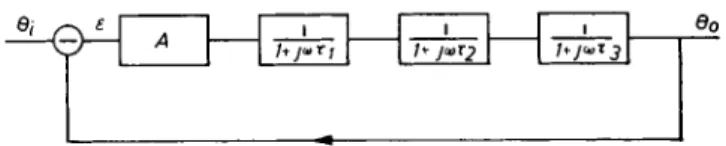
C. One of the means of realizing an apparently larger xx is the use of a so-called "phase-lag network". This is an electrical (or pneumatical) net
work with a frequency response function:
y _ 1 + > τ Β
χ 1 + Β]ωτΒ'
When choosing τΒ = τΐ9 the factor 1 1 +J£ori
representing the influence of the largest time-constant in the open-loop characteristic, is replaced by a factor
1
1 + Bju>%i
So the system will behave as if the largest time-constant were Βτλ. This means that the loopgain may be raised by a factor Β as well (Fig. 6).
(B-I)R
GQ.AB - ε "
θρ___Α -
Fig. 6. Fig. 7.
Fig. 6.—Correction with a phase-lag network.
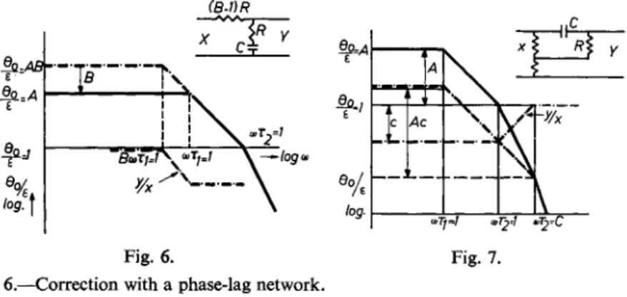
Fig. 7.—Correction with a phase-advance network.
D. In a similar way τ2 can be reduced by the use of a phase advance net
work, with a frequency response function:
This type of network sometimes is referred to as a damping network, be
cause of its damping effect in the closed loop (when properly used). Here rc must be chosen equal to τ2, with the result, that in the open-loop characte
ristic τ2 is replaced by r2/C, and the loopgain may be enlarged with a factor
The results are essentially the same as when τ2 really is made smaller, but there is one difficulty more: the filter gives a D.C. attenuation of a factor C, so that an additional amplification factor C is necessary. Some
times this can give rise to noise problems.
In practice Β and C have an order of magnitude of 10. Essentially the same effects as described under paragraphs C and D can be reached when integrating and differentiating action are incorporated in the controller:
E. In a ΡΙ-controller the deviation ε is not only amplified but in the same time it is integrated with respect to time. The response function of a P I - controller therefore is:
χ C \+(j(oxclC)'
C ( F i g . 7).
εάΐ
or, for sinusoidal signals:
N o w integrators in practice are seldom real integrators (the amplification-
11-60143045 I & Μ
factor for D.C. signals is not infinite but bx,, b> 1). Therefore the frequency response function is in fact:
y = A l+jcoTj =^bl + b j a> r i
ε l/b+jcoTi l+bjcoTi'
This is exactly the same formula as can be derived for a phase-lag network.
When chosing xt = τΐ9 xx is replaced virtually by bxx. The difference with a phase-lag network is that b in most cases can be chosen considerably higher than Β in phase-lag networks.
F. PD-controller. In principle here is y = Α (ε + rd[de/dt]) or, for sinus
oidal signals: y/ε = A(l + j c o Td) . Here, too, there is a practical limit, real differentiators stop differentiating at a certain high frequency, and therefore a more realistic expression is:
ε 1 + ]ω %a\c
This is the same function as was derived for a phase-advance network, again xd should be made equal to τ2. The only difference with a phase- advance network is that c in most cases is considerably higher than C.
Both c and b are in the order of magnitude of 100x.
In each individual case it will be necessary to decide which of the above- mentioned methods will be most suitable. Of course a combination of two or more is always possible for further improvement of the control quality.
The best known combination is the PID-controller. Here xx is made larger by the integrating action and τ2 is made smaller by the differentiating effect.
From the preceding discussion it will be clear that the right setting of a PID-controller should be xt = xl9 xd = τ2. This in itself is already a rule that can easily be observed and proves to give good results in many cases.
In this paper we have tried to make clear that all methods, well known in normal control practice, to improve the quality of the feedback loop, become natural and trivial means, when the formula A = Χχ/χ2 (derived for an idealized case) is used as a starting point. For a proper appreciation of the value of the different methods possible and their mutual connection, this can be of great help to students in control theory.