C O M P A R T M E N T A L A N A L Y S I S A N D T H E T H E O R Y O F R E S I D E N C E T I M E D I S T R I B U T I O N S
R U T H E R F O R D A R I S
Department of Chemical Engineering, University of Minnesota, Minneapolis, Minnesota
T h e following survey touches on two areas of s t u d y t h a t h a v e rele- vance to biological problems. T h e y h a v e been opened u p to some extent by m a t h e m a t i c a l analysis, a n d though the results are not y e t applicable in t h e detail t h a t one would like to a t t a i n , t h e y do furnish some grounds for hope in t h e fruitfulness of a cooperation between t h e biologist and chemical engineering scientist.
T h e first area is k n o w n to t h e biologist as t h e theory of t r a c e r methods a n d c o m p a r t m e n t a l analysis, and a large a m o u n t of biological work of v a r y i n g degrees of sophistication has grown up in it. I t is almost precisely paralleled by t h e t h e o r y of residence t i m e distribu- tions a n d the analysis of first-order kinetics developed by chemical engineers, but, u n f o r t u n a t e l y , like almost parallel surfaces t h e two areas h a v e seldom been in contact. H e r e t h e biologist m a y be inter- ested to learn w h a t m a y be said in rigorous b u t quite general t e r m s a b o u t t r a c e r m o v e m e n t s a n d to see an entirely different a p p r o a c h to c o m p a r t m e n t a l analysis. T h e engineer needs to become a c q u a i n t e d with the complexity of biological problems and to get something more t h a n a superficial knowledge of the subject before he can m a k e a really useful contribution.
T h e second area m a y be described as a group of m o d e r a t e l y com- plex problems whose solutions can be expressed in relatively simple t e r m s . These problems are of course of a m u c h lower order of complex- ity t h a n t h a t of biological systems, b u t it is still sufficient to give in- centive for t h e development of simplifying methods, a few of which are sketched here.
F i n a l l y it m a y be r e m a r k e d in the p a r t i c u l a r context of this con- ference, t h a t the t e r m "residence t i m e " m a y be replaced by " t r a n s i t t i m e , " so t h a t some of the methods outlined are of i m m e d i a t e applica- tion to t r a n s p o r t problems.
167
168 R U T H E R F O R D A R I S
L E A R N I N G A B O U T S I Z E S , R A T E S , A N D F L O W P A T T E R N S
The Theory of Residence Time Distributions The Ideal Tracer Experiment
T o fix our ideas on something reasonably general b u t quite definite, let us consider t h e problem of flow through a container. W i t h i n this container a mixing or exchange process is t a k i n g place of which we w a n t to learn as much as possible by some t r a c e r experiment. To the obvious question, " H o w long does a p a r t i c u l a r molecule spend in t h e c o n t a i n e r ? " there is t h e obvious answer, " I t v a r i e s , " a n d t h e i m m e d i a t e consequence t h a t we need a p r o b a b i l i t y distribution to describe t h e system. If we t h e n ask, " W h a t is t h e p r o b a b i l i t y t h a t a molecule will spend a time between t and t -f- St in t h e s y s t e m ? "
we see t h a t this could be answered by t h e idealized experiment of instantaneously injecting a q u a n t i t y of tracer a t time t = 0 a n d m e a - suring its concentration in t h e effluent. L e t c(t) be this concentration a t time t, t h e n c(t) dt is proportional to t h e n u m b e r of molecules emerging a n d / c(t) dt is proportional (with the same constant of proportionality) to t h e t o t a l n u m b e r injected. Since this is in fact a very large n u m b e r we h a v e in the ratio
as good a n approximation to t h e frequentist definition of p r o b a b i l i t y as we are likely to find. T h e function p(t) so obtained is therefore the p r o b a b i l i t y density function for residence time within the system.
A certain a m o u n t of information a b o u t the system is contained in this function p(t). Indeed, by calculating t h e behavior of some ideal systems we m a y see how to interpret such a function. D a n c k - werts [8] was t h e first t o explain this in chemical engineering t e r m s and to suggest even simpler p a r a m e t e r s t h a t might usefully c h a r a c - terize t h e distribution. T h e obvious p a r a m e t e r s are t h e m o m e n t s of the distribution. T h u s the expected value of t h e residence t i m e is
( 1 )
(2) and its v a r i a n c e is
(3)
C O M P A R T M E N T A L A N D R E S I D E N C E T I M E A N A L Y S I S 1 6 9
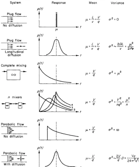
FIG. 1. T h e response of various systems to an ideal tracer experiment.
These two n u m b e r s are of t h e first i m p o r t a n c e t h o u g h t h e y are far from complete characterization of t h e residence t i m e distribution for which t h e complete set of m o m e n t s
mk = fj t k
p(t) dt, k = 1, 2 . . . (4) would be needed. ( N o t e : ra2 = μ
2 + σ
2 .)
Figure 1 shows t h e p r o b a b i l i t y densities arising from some simple
System Response Mean Variance
170 R U T H E R F O R D A R I S
systems. W h e n t h e equilibrium concentration distribution of c throughout the system would be constant a n d equal to a constant feed concentration, t h e m e a n residence time is the t o t a l volume over t h e volume flow-rate, a t least a s y m p t o t i c a l l y . T h i s result is proved in the appendix in a slightly more general situation. T h e v a r i a n c e is related to the intensity of mixing or a m o u n t of diffusion in the system. T h u s m e a s u r e m e n t of t h e m e a n and variance of residence times gives some information a b o u t the system, as the physiologist a c q u a i n t e d with dye-dilution techniques well knows.
Residence Time and Age Distributions
An a l t e r n a t i v e w a y of describing t h e residence t i m e is t h e probabil- ity distribution function
Pit) = /„ PU') dt' (5) P ( i ) is t h u s t h e fraction of molecules t h a t spend a time of t or less
in t h e system. Conversely,
pit) = dP(t)/dt (6) Also
μ
= fjt pit) dt= -J
0~
td[l
= [ - « { 1 - Ρ « ) Π ο + / „ " i l
= fj i l - Pit)} dt
This is shown in Fig. 2. D a n c k w e r t s , who first showed t h e usefulness of these concepts in chemical engineering situations [ 8 ] , also sug-
- PH)} (7) - Pit)} dt
C O M P A R T M E N T A L AND R E S I D E N C E T I M E A N A L Y S I S 171 gested t h a t the p a r a m e t e r
H
= $fo
Pit)dt =Q)l"
{l-
Pit)]dt (8)which he called the hold-up, would be a useful measure of t h e presence of mixing or diffusive dispersion.
Another i m p o r t a n t distribution is the internal age distribution.
I(t) dt is the fraction of molecules within the system t h a t have been there for a time between t and t -f- dt (i.e., are of age t to t-\-dt).
If there are Ν molecules per unit volume, then of t h e Nq dt t h a t en- tered the system between times zero a n d dt, VNI(t) dt are still there at time t and Nq dt P(t) h a v e a l r e a d y passed out. Hence
q = VI(t)
+
qP{t)/ « ) = f { 1 - ^ ( 0 } (9) T h e average age of molecules within t h e system is
tl(t) dt = ^ fj 2t{l - P(t)} dt = ^Jj t*p(t) dt
2V 2μ
κ ι υ
)
We observe t h a t
Η = I(t) dt (11) T h e hold-up Η is a measure of the d e p a r t u r e from piston or plug
flow. D a n c k w e r t s also suggested a m e a s u r e of t h e d e p a r t u r e from complete mixing in the area of one of t h e lobes between the complete mixer curve P(t) = 1 — e~
t,fi
and a given distribution, i.e.,
S = ifj\l - e""* - P(t)\ dt (12) T h e "segregation" S is given the sign t h a t {1 — e~
f/
^ — P(t)} t a k e s for sufficiently small values of t (Fig. 3 ) .
These p a r a m e t e r s describe the s t a t e of mixing within the system by giving some indication of how the residence time is distributed.
T h e concepts introduced by D a n c k w e r t s h a v e been found useful in the analysis a n d design of reactors a n d also in t h e s t u d y of a n u m b e r of chemical processes. Before comparing this with t h e biological a p -
172 R U T H E R F O R D A R I S P(t)
FIG. 3. Illustrating the notion of segregation.
proach one or two points a b o u t t h e analysis of t r a c e r experiments should be m a d e .
The Analysis of Tracer Experiments
Consider two simple special cases of the general situation p o r t r a y e d in t h e appendix. I n Figure 4a, we h a v e a fluid flowing
P(t)
(a)
— E ^ t —
P(t)
(b)
FIG. 4. T h e effect of retention of the tracer by the wall of the system.
uniformly down a t u b e with a v e r y small a m o u n t of longitudinal diffusion present. T h e P(t) distribution is therefore a v e r y sharp step a t t h e m e a n residence time μ] if there were no diffusion it would be perfectly s h a r p . T h e m e a n residence time is the volume of the t u b e divided b y t h e volume flow r a t e or, equivalently, the length of t h e t u b e divided by t h e linear velocity of flow. I n Figure 4b, t h e tube is coated with a t h i n layer of a second phase (e.g., silicone) into which t h e tracer can be absorbed; indeed, it is essentially a coated-tube chromatographic column. W i t h the same length of tube and same linear velocity the m e a n residence time is now increased
COMPARTMENTAL AND RESIDENCE T I M E ANALYSIS 173 by a factor of (1 -f « ) , where a is t h e r a t i o of t h e a m o u n t of t r a c e r t h a t would be held in the coating in equilibrium with a uniform con- centration in the t u b e to t h e a m o u n t so contained in t h e free space of t h e t u b e . T h u s an experiment of this k i n d does give t h e m e a n residence time of the tracer, b u t unless t h e retention of t h e t r a c e r on the wall is explicitly recognized, it would lead to an incorrect estimate of t h e free volume of t h e t u b e . T h e same situation occurs if t h e tracer is not carried in the s t r e a m b u t on some bodies n o t moving with exactly the same speed—as, for example, with a t r a c e r held on the red cells in p l a s m a ; this is sometimes referred to as
"slippage."
T h e slope of the b r e a k t h r o u g h curve depends on t h e diffusion p r o - cesses; if there is little longitudinal diffusion in t h e flowing s t r e a m the P{t) curve will be quite s h a r p in t h e first case. I n t h e second case it depends also on the r a t e of exchange between the s t r e a m a n d the coating and possibly upon diffusion within t h e coating. T h e diffu- sive processes do h a v e a small effect on t h e mean residence t i m e but this is a s y m p t o t i c a l l y negligible.
Another assumption m a d e in calculating volume from such a t r a c e r experiment is t h a t all tracer passes into t h e system a n d t h a t t h e r e is no back-diffusion against t h e perfusing stream. Spalding [14]
showed t h a t if t h e area of t h e incoming s t r e a m were A% a n d t h e diffusion coefficient in it were D ; , then the m e a n residence time would not be μ = V/q b u t
V DiAi
2
„ = + — (13) I n chemical engineering experiments the conditions can often be con-
trolled to m a k e this second t e r m small, b u t this m i g h t n o t a l w a y s be so easy in biological contexts. I n principle it m i g h t be allowed for by perfusing a t two different rates, say q a n d Xq (λ > 1 ) . T h e n
V , DiAi* V , DiA. .2 μ = 1q q 2— > Μλ = τ - +
2 ^
A
Xq X 2
q
2
a n d
V/q = (λ 2
μχ ~ μ ) / ( λ - 1) (14) A more significant point to note is t h a t ( a p a r t from small correc-
tions) it is n o t i m p o r t a n t t h a t t h e t r a c e r should be injected in t h e
" i d e a l " w a y described above. T h e m e a n residence t i m e is t h e difference
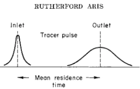
174 R U T H E R F O R D A R I S Inlet Outlet
Tracer pulse
Mean residence — time
FIG. 5. Response of a system to a nonideal injection of tracer.
between t h e mean times of t h e inlet a n d outlet distributions of concen- t r a t i o n as shown in Fig. 5.
Some Biological Tracer Experiments
I t would p r o b a b l y surprise t h e chemical engineer to learn t h a t some pioneer work on t r a c e r methods in biological systems dates back to 1931 a n d even anticipates some of his latest suggestions (cf. D a n c k - werts' r e m a r k s in the discussion of Klinkenberg's p a p e r [12] a n d H a m i l t o n ' s correction for recirculation), b u t t h e substance of t h e sec- tion under t h e heading of t h e S t e w a r t - H a m i l t o n principle in Shep- p a r d ' s book on t h e t r a c e r method does in fact anticipate engineering applications by more t h a n t w e n t y years. P e r h a p s t h e engineer m a y contribute a little by showing how t h e theoretical basis of t h e method is established—it is in fact applicable under fewer restrictions t h a n those Sheppard gives—and b y suggesting how other features of interest could be elucidated from suitable experiments.
If, as above, t h e concentration of a certain tracer in the effluent stream is c(t) t h e t o t a l a m o u n t t h a t emerges is
where q is the volumetric flow r a t e , assumed constant. If a known a m o u n t , C0, was injected and there is no diffusion behind t h e injection point then this integral m u s t equal C0 and so
If q is a monotonie function of time this formula will give an average value. T h e integral is over an infinite i n t e r v a l a n d so m u s t be t r u n c a t e d . H a m i l t o n [10] suggests t h a t t h e form of t h e tail will be c(t) oc β ~
λί
and there is every reason to suppose t h a t this is so, though a complete proof h a s y e t to be given for t h e general case. If t h e d a t a are plotted on logarithmic p a p e r a n d it becomes plain t h a t t h e curve
c(t) q dt
(15)
C O M P A R T M E N T A L AND R E S I D E N C E T I M E A N A L Y S I S 175 is a s t r a i g h t line beyond t h e time t = t0 so t h a t c(t) = c(t0) e"
> ( i
~ i
«.
) , with λ determined by t h e slope of t h e line, then
/0°° c(t) dt = | J ° c(t) dt + c(U)/\ (16) If there is no " s l i p p a g e " the measured m e a n residence time gives
the volume V = q, where
μ = fj t c(t) dt = t c(t) dt + c(*0)(l + λ /0) / λ 2
(17) P r o v i d e d t h a t λ can be determined before t h e effect of recirculation is felt, this provides an a d m i r a b l e method of correcting for recirculation.
One of t h e assumptions on which t h e v a l i d i t y of this method is established is t h a t the tracer is uniformly distributed across t h e incom- ing vessel. T h e precise correction t h a t m u s t be m a d e when this is not the case is difficult to determine ; an e l e m e n t a r y example is given in some detail b y Aris [ 1 ] . I t is an a s y m p t o t i c a l l y small correction in t h e sense of being independent of volume, whereas t h e m e a n resi- dence time is proportional to volume. Another assumption (mentioned above) is t h a t there is no back-diffusion a t t h e inlet. E q u a t i o n (14) gives a method of correcting for this. T h e assumption t h a t t h e influent s t r e a m m a y be broken up into a n u m b e r of fractions each of which traces a certain p a t h through t h e l a b y r i n t h w i t h o u t a n y real com- munication with its fellows (and some such assumption lies behind the proof commonly given if t h e relation ^q = V) is n o t necessary.
If, however, it is justifiable we can get r a t h e r more information out of t h e residence t i m e distribution t h a n t h e m e a n affords. This concept of individual p a t h s — s o m e t i m e s called " s t a b l e " — i s of course an ideali- zation, b u t h a s been proposed by T u r n e r [17] as a model for t h e packed bed. Consider a single p a t h of length I along which t h e volume flow r a t e is q(l) and t h e linear velocity u(l). T h e L a p l a c e t r a n s f o r m of the concentration pulse a t the exit in t h e ideal t r a c e r experiment is
* ( l , p ) « l -
P( £ ) + gP'
/2
Dl D 2
\
/2
where D is the longitudinal diffusion coefficient in the fluid. T h e last two terms can be w r i t t e n
2 ^ {1 - (1 - e-^
D
)/(ul/D)}
176 R U T H E R F O R D ARIS
and if the dimensionless group ul/D (a so-called Peclet or Bodenstein number) is large the second term is small. If we sum the responses over each length of path we have the weighted mean
Σς(1)ο(1,ρ) = 1 _ ?kQ)/u{})_
?q(l)
y 2q(l)
1 Vq(l){[l/u(DY + [2Dl/u:(D]\
~^2 V
?q{l) Now q(l) = A(l)u(l) where A(l) is the area of a channel of length I a n d %IA{1) = V; thus the coefficient of — ρ is (V/q) = μ, as we should expect. T h e coefficient of | p
2 is (σ
2 + μ
2
) and hence
The first term is contributed by the ultimate mixing of streams which have taken different times to pass through the system. T h e second term is the effect of diffusion within each channel.
In principle, the two terms can be distinguished and the second one analyzed as follows. If the same pressure drop obtains over each channel the linear velocity will be related to the area and length by
u{l) = ώΑ(1)/1 (20) where ώ is a constant proportional to the pressure drop and dependent
on the viscosity of the fluid and the shape of the channels. The constant ώ is related to the total flow rate by
q = Σβ(Ζ) = ώ Σ A (I)/I, (21) so that the firm term in E q . (19) may be written as MV
2 /q
2
, where
M = {ΣΙ*} {Σ^ψ\/{ΣΙΑ(1)\* - 1, (22)
a factor which depends only on the geometry of the bed. If the disper- sion in the channel is the result of molecular diffusion and convection, then D m a y be related to t h e molecular diffusion coefficient Dm by Taylor's formula (see section on Taylor Diffusion in Use of M o m e n t s ) .
D = Dm + KA(l)u 2
(l)/Dm, (23)
C O M P A R T M E N T A L A N D R E S I D E N C E T I M E A N A L Y S I S 177 where κ is a factor depending on t h e shape of t h e channel a n d flow profile. If this is s u b s t i t u t e d in E q . (19) we h a v e
σ 2
= LM + Μ μ 2
+ Νμ* (24)
where
_ 2κ {ΣΙΑ*(1)} . L
~ W m [ZIA(J)\ W
a n d
\ΣΙ>/Α(!)}{ΣΑ*(1)/1\*
Ν = 2D„
{ΣΙΑ(1)}
T h e coefficients L and M depend on t h e flow and diffusion coefficient as well as t h e geometry of the bed. T h e r e does seem to be t h e possibil- i t y here of distinguishing t h e t h r e e t e r m s or a t least e s t i m a t i n g their i m p o r t a n c e b y t r a c e r experiments a t a n u m b e r of different flow r a t e s , a n d we should like to raise t h e question of w h e t h e r this h a s been exploited in biological e x p e r i m e n t a t i o n . T h i s model m a y be generalized to a n y distribution of length area and shape of channel. [4, 5 ] .
First-Order and Exchange Processes
T h e uniform, spontaneous d i s a p p e a r a n c e of t r a c e r from a system as if b y a first-order reaction can be a n a l y z e d r a t h e r easily. A first- order process represents a spontaneous event, i n d e p e n d e n t of o t h e r s ; if t h e p r o b a b i l i t y of this h a p p e n i n g in a n y i n t e r v a l (t, t + St) is k St, where k is a constant, t h e p r o b a b i l i t y of a molecule surviving this t r a n s f o r m a t i o n from time 0 to t i m e t is exp-kt. Since p(t) dt is t h e p r o b a b i l i t y of residing in t h e system for a t i m e between t and t -f- dt, t h e expected value of the survival p r o b a b i l i t y is
€ = E(e- kt
) = fj e~
kt
p(t) dt (26)
T h i s formula m a y also be established from t h e differential e q u a t i o n as is shown in t h e appendix. Clearly, e is a function of k a n d in fact m a y be o b t a i n e d i m m e d i a t e l y from t h e L a p l a c e t r a n s f o r m e d equations of t h e system with b o u n d a r y conditions for t h e ideal t r a c e r experiment ; e is also a functional of t h e p r o b a b i l i t y density p(t) a n d so a function of its p a r a m e t e r s (i.e., m o m e n t s ) .
I n chemical engineering contexts it is common t o compare e w i t h
178 R U T H E R F O R D ARTS
t h e two extreme situations of piston flow, p(t) = 8(t — μ), a n d a single c o m p a r t m e n t p(t) = exp (—ί/μ)/μ. These give respectively
ei = e-** a n d e
2 = (1 + μ/c)- 1
(27) and
00
L
=f -*«-*>
e p(<) dt = l+ + V Ρ- (
2 8)
3
where pn is t h e r a t i o of t h e nth m o m e n t a b o u t t h e m e a n t o σ η
. T h i s convenient dimensionless form sometimes gives a s e t of n u m b e r s independent of μ or σ a n d t h u s m a k e s t h e r a t i o c/ci a function of ak only. F o r example, the Gaussian distribution gives p2n = {2n)\/2
n n\
P2n+i = 0, and hence
6 V (*
k
)*
n
1 27 2 - = / - ~ — r = e x p ±a
2 k
2
71 = 0
T h e residence time distribution of Ν c o m p a r t m e n t s of equal size in series is
fN-l /Λ7\ Ν
^ - ( Λ Γ = 1 ) ί ( ^ ) <-"«>
giving
i -
ek> (
l +¥)'"=
EXP(FARARI)0 + %)'"
since t h e variance σ 2
= μ/Ν.
If t h e first-order process is not uniform the general equation cannot be so easily solved. F o r a one-dimensional flow, as in a channel of v a r y i n g section, with linear velocity, u(z), and r a t e constant, k(z), functions of distance from the inlet, t h e concentration of t r a c e r would be given by
^M
+ M(,)^) = -
f c(,
) c M(29)
W i t h c(z,0) = 0 and specified c(0,t) — Cf(t), t h e solution is
c(z,t) = cf(t — r ) exp — kr (30)
C O M P A R T M E N T A L A N D R E S I D E N C E T I M E A N A L Y S I S 179 where
r =
ο u(x)2
dx a n d kr = k(x) dx
u(x) (31)
I n t h e distributed model of the exchange with an environment, where the r a t e of exchange is finite, t h e equations and their solutions can become very complicated. T h e r e is an analogy here to t h e theory of h e a t exchangers and of c h r o m a t o g r a p h y . Some references are given below.
Tracer Experiments with Other Signals
M e n t i o n should be m a d e in passing of another technique t h a t chemical engineers h a v e used in analyzing complex systems. I t was pioneered by R. H . Wilhelm and his students and uses an i n p u t tracer concentration t h a t fluctuates sinusoidally (see [ 2 1 ] ) . B y observing the a m p l i t u d e ratio and shift of phase m u c h information a b o u t t h e internal r a t e processes of the system can be obtained. T h i s method is clearly related to the impulse tracer experiment, j u s t as the two methods of describing control mechanisms (by impulse weighting func- tions and frequency response) are related. Indeed, by t h e convolution theorem t h e response to an i n p u t v a r i a t i o n F(t) = a -f- b cos ωί is
G(t) = p(s){a + b cos œ(t — s)} ds
and afte r a lon g tim e thi s tend s t o
G(t) = a jQ p(s)ds + b co s œt jQ p(s) co s co s ds
(32)
= a + ab co s (ωΐ — φ) (33)
where
,2 _
I/o" P«
cos cos dsand
φ = t a n -1
Clearly, if t h e a m p l i t u d e r a t i o a a n d p h a s e shift φ are k n o w n as functions of ω, t h e impulse response can be reconstructed. Correspond- ingly, if p(t) is known, the frequency response can be predicted.
180 R U T H E R F O R D A R I S
Compartmental Analysis
The General Problem and Its Relation to Chemical Kinetics I t is interesting t h a t the c o m p a r t m e n t a l analysis of t h e biologist has its greatest affinity with t h e chemical kinetic studies of engineers r a t h e r t h a n with residence t i m e distribution analysis. B y c o m p a r t - m e n t a l analysis I u n d e r s t a n d t h e following general problem t o be m e a n t (Sheppard [ 1 3 ] , C h a p t e r 3 ) . Ν c o m p a r t m e n t s are interconnected in such a w a y t h a t t h e t r a n s p o r t r a t e of m a t e r i a l into c o m p a r t m e n t i from c o m p a r t m e n t ; is pij. T h e t o t a l a m o u n t of a labeled species in c o m p a r t m e n t i is Si a n d its specific a c t i v i t y α^, so t h a t t h e t o t a l activ- ity is Ri = Siai. T h e equations governing Si a n d Ri are
a]Si dt
IS J\ J\
= ^ Vij -
X
Va =X
(Vi3 ~ Vh(35) a n d
Ν
-1 ,- = 1
=
~
ΑΊX
V J I +X
P I J A J =X (
PIJA* ~
Ρ3ΊΑ^ ^
3 = 1 ,- = 1
3 = 1
where i t m a y be understood t h a t pa = 0.
Ν Ν Ν B U T
X ^ f
=X X ( p « - p - ) = o
i=l i=l,-=1
Ν Ν Ν
and Χ
=X X (
PI3'
A' ~~
VJIA^
=°
i=l i=l j=l
so t h a t a t most (N — 1) of each of these sets of equations can be inde- pendent. T h e object of t h e exercise is t o determine t h e iV sizes, Si, a n d N(N — 1) exchange r a t e s pij.
T h e method proposed m a y be illustrated by t h e case where the c o m p a r t m e n t sizes are a l r e a d y known and Ν different t r a c e r s m a y be used; then for the r
th
t r a c e r we have a specific a c t i v i t y r
a j and t o t a l activity
r Ri a n d
Ν
(pifdj - pji'cii) = j r
Ri = r
Ri (37)
C O M P A R T M E N T A L A N D R E S I D E N C E T I M E A N A L Y S I S 181 are t r e a t e d as a set of simultaneous equations for t h e u n k n o w n s pij.
T h e solution is where
Δ =
pjk = Ajk/A (38)
1
Cti ' ' ' ·
l
dN
(39)
a n d Ajk is the d e t e r m i n a n t obtained by replacing t h e fc th
column of Δ b y
x Rh . . .
N Rj.
Unless it is possible to m a k e easy a n d a c c u r a t e m e a s u r e m e n t s of the
r cii a n d
r
Ri and to o b t a i n reliable estimates of t h e derivatives of t h e latter, it is unlikely t h a t this m e t h o d would give accurate results. I n this case it is not clear w h y it would not be simpler to t a k e Ν observations of one tracer in preference to Ν tracers. Sheppard shows later in his book the importance of careful fitting in t h e e s t i m a - tion of constants. An i m p o r t a n t m e t h o d a n d one t h a t is capable of considerable refinement is to compare t h e experimental observations with t h e values calculated from the solution of t h e differential e q u a - tions with a t r i a l set of t h e p a r a m e t e r s , pij. These are t h e n adjusted until t h e sum of t h e squares of the differences is minimized. T h e method can be sophisticated so t h a t confidence limits on the estimates of the p a r a m e t e r s can be obtained.
I t is interesting to compare the kineticist's a p p r o a c h t o t h e same problem as exemplified in Wei a n d P r a t e r ' s w o r k on monomolecular reactions. T h e method m a y be seen m o s t easily by considering t h e t h r e e - c o m p a r t m e n t case. T h e equations for t h e specific activities in three c o m p a r t m e n t s of size Si, S2, and S3 are
* - 1 1 ( 1 ) * -(!')«•
, = 1 3
i = l
3
where pi/ = Pa/Sj. Since ^ Ri is c o n s t a n t we can represent t h e i = l
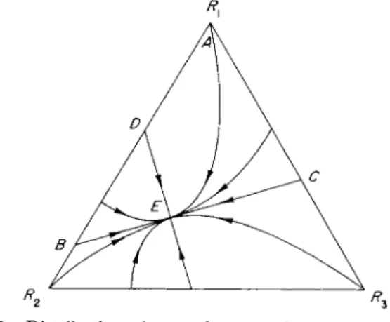
s t a t e of t h e system a t a n y time as a p o i n t in a t r i a n g u l a r d i a g r a m such as Fig. 6. As time goes on the point moves to its final equilibrium
182 R U T H E R F O R D A R I S
position in which t h e tracer is uniformly distributed t h r o u g h o u t t h e system. F o r example, if all the tracer is initially in c o m p a r t m e n t 1 (i.e., t h e initial s t a t e is represented by point A) t h e history of the distribution might be represented by the curve AE. This curve approaches Ε t a n g e n t i a l l y to a certain fixed direction BEC, which cannot be determined accurately but can a t least be estimated by plotting the observations of Ri in the diagram. B y trial and error t h e initial distribution of tracer between c o m p a r t m e n t s 1 and 2 cor- responding to the point Β m a y be found, such t h a t the observations fall on a straight line BE. This is quite a sensitive test and if t h e logarithm of the distance from Ε is plotted against time it will be
FIG. 6. Distribution of tracer between three compartments.
found to give a straight line with slope corresponding to the largest nonzero eigenvalue of t h e system, which can t h u s be determined very accurately. T h e second eigenvalue can be found by finding the other p a t h DE, which is a straight-line p a t h , but to which the other p a t h s are not t a n g e n t . T h e full algebraic details of this are contained in Wei and P r a t e r ' s long article in Advances in Catalysis, and other simplified expositions exist [7, 19, 2 0 ] .
T h e p r a c t i c a b i l i t y of this m e t h o d depends on how easy it is t o repeat experiments with different initial distributions of tracer between the c o m p a r t m e n t s .
The Simple Catenary and Its Limiting Cases
T h e simple c a t e n a r y of c o m p a r t m e n t s in which pi+1,i = pi
<p{. = 0, j 9* i — 1, is susceptible of a p a r t i c u l a r l y simple analysis.
C O M P A R T M E N T A L AND R E S I D E N C E T I M E A N A L Y S I S 183
F o r t h e ith c o m p a r t m e n t
Si ^~ = ρ<_ιθΐ_ι — pidi (40) and hence
a,i(t) = <ii(0) exp — pd/Si
+ (pi-i/Si) J* α»_ι(ί - s) exp (-pis/Si) ds (41) If E q . (40) is w r i t t e n
dcti Pi^! , , pi — pi_i , N
-jj + Z g - (a* - a , _ i ) = -
^ a{ (42) s
it will be seen to be the discrete analog of E q . (29) with u(z) cor- responding to p i - i / S i and k(z) to {pi — pi-^/Si.
If there is interchange in both directions between adjacent c o m p a r t - ments, i.e., Pij = 0 if i — ; ^ 1, we h a v e t h e equation
^ i
~aY =
P ^ - 1
^ - 1
~~ (Pi-is + Pi+hi)ai + pi,i+iai+i (43) An e l e m e n t a r y solution is not obtainable for this except under certain simplifying assumptions. B y writing this equation in t h e form ddi (Pi,i-1 + Pi,i+l\ On -L. η \ ( ~ Ρ^+Λ it = \ — 2 ^ — ;
{ αι ί + -
2 ι +α a i -
i]
- \ — & — )
X i {ai +1 - a^\ - " + *™ ' ^ ai we see i m m e d i a t e l y t h a t there is an analogy with t h e diffusive
equation
ft
=
™S -
u^
f - ^ c ^ kAgain this e q u a t i o n is m u c h less easy to solve t h a n the first-order E q . (29).
Continuous Compartmental Analysis
T h e general equations of c o m p a r t m e n t a l analysis are analogous to the equations of first-order reactions in continuous mixtures, which h a v e been considered elsewhere [ 9 ] . I n a continuous m i x t u r e (or a continuous spectrum of c o m p a r t m e n t s ) we can no longer distinguish individual species (or c o m p a r t m e n t s ) , b u t designate t h e m by a con-
184 R U T H E R F O R D A R I S
tinuous variable χ over a finite interval ( a , 6 ) . T h e concentration of the "species" in t h e infinitésimal interval {χ. χ -\- dx) (or in t h e in- finitesimal c o m p a r t m e n t (χ, χ + dx) is c(x,t) dx. T h e equation of change analogous to E q . (36) is now an integrodifferential equation.
T h e solution of this equation depends on t h e n a t u r e of t h e kernel function k{x,y), which gives t h e r a t e of exchange into t h e c o m p a r t - m e n t {χ, χ -f- dx) from {y, y + dy). I t is linear so t h a t t h e Laplace t r a n s f o r m a t i o n m a y be used, but the inversion requires a fairly deli- cate consideration of the spectrum of the operator
S I M P L E D E S C R I P T I O N S O F C O M P L E X S Y S T E M S
I wish to present in this section a few examples of the w a y in which quite complex situations h a v e been presented in v a s t l y simpli- fied, but useful, ways. These are related to w h a t h a s gone before where some of the same techniques, including the method of moments, have been used. F i n a l l y , I should like to a d u m b r a t e a t h e o r y of diffu- sion in continuous mixtures.
Taylor Diffusion
I t is interesting to observe t h a t of some two hundred references to papers in Sheppard's "Basic Principles of the T r a c e r M e t h o d , "
p r o b a b l y only one would be recognized by the average chemical engi- neer. This is Sir Geoffrey T a y l o r ' s analysis of " t h e dispersion of solu- ble m a t t e r in a solvent flowing slowly through a t u b e " [ 1 5 ] , itself provoked by unproved assumptions in earlier work, some of it biologi- cal. I n this p a p e r T a y l o r considered the difficult problem of combined diffusion and l a m i n a r flow a n d showed t h a t t h e interaction of these two effects could be w r a p p e d u p in an a p p a r e n t diffusion coefficient of a
2
£ / 2
/ 4 8 D , where a is t h e r a d i u s of t h e t u b e ; U, the m e a n velocity;
w h e r e (46)
(45)
{p + K(x)} + j b
ak{x,y)
The Use of Moments
C O M P A R T M E N T A L A N D R E S I D E N C E T I M E A N A L Y S I S 185 a n d D , t h e molecular diffusion coefficient. T h e factor T^ is characteris- tic of t h e shape of t h e cross-section of t h e t u b e a n d of t h e flow profile.
T a y l o r ' s m e t h o d of deriving this result w a s also c h a r a c t e r i s t i c ; he employed his great physical insight to see w h a t t e r m s could be n e - glected a n d produced a method of astonishing simplicity. I t is almost a p i t y to sophisticate such work, b u t t h e use of m o m e n t s does allow a little more to be said without too much extra complication.
F o r this purpose we consider t h e spatial m o m e n t s in a n infinite t u b e r a t h e r t h a n t h e t e m p o r a l m o m e n t s t h a t arise in t r a c e r experi- ments. If χ is a coordinate along t h e axis of t h e t u b e a n d y a n d ζ coordinates in t h e plane of cross-section t h e velocity profile can be w r i t t e n u{y,z) = U[l -\-χ(ν,ζ)] in t h e domain S of t h e cross-section, χ being a function with zero m e a n value. Similarly t h e diffusion co- efficient m a y v a r y over t h e cross-section a n d we write D(y,z) — Dij/(y,z). C(x,y,z,t), t h e concentration of solute a t a n y point a n d time, satisfies
i f = V(*VC) - g (1 + χ ) f (47) I t is convenient in these flow problems t o t a k e a moving origin (in
this case one moving with t h e m e a n speed of t h e s t r e a m ) a n d t o m a k e the physical quantities dimensionless. T h u s if
ξ = (x - Ut)/a, η = y/α, f = ζ/a, τ = Dt/a 2
, μ = Ua/D (48) the equation for C becomes
dC dr
, d 2
C d ( dC\ , d ( dC\ dC
and is subject to t h e initial condition
c(i,u,r,o) = c
0(f,i7,r) (50)
and the b o u n d a r y condition
* ^ = 0 (51) ov
where d/dv d e n o t e s differentiation n o r m a l t o Γ, t h e b o u n d a r y of S.
W e define s p a t i a l m o m e n t s b y
and
C
P(v,M
= ?C(MT)dt
(52)™>P(T) = / /
Cpdvdç/ j !
άηάξ (53)186 R U T H E R F O R D ARTS
This allows somewhat simpler differential equations to be written down for cp and mp of which we shall only quote
dm,
d p(p - 1) l^CP_2 + ρμ x cp_ i (54) the bars denoting an average over the cross-section. Thus we get
immediately t h a t m0 is constant and to obtain
ύυι
ύ we must solve for c0. I t turns out t h a t c0 is a constant plus exponentially decaying terms and since it is multiplied by χ (whose mean is zero) before being averaged over the cross-section it contributes only exponential terms to dm1/dr. Thus m1 tends to a constant as time increases and this means t h a t the center of gravity of the solute does move with the speed of the stream. Its ultimate displacement from the moving origin is a function of the initial distribution. By solving for cx and substituting in Eq. (54) it can be shown that~ 2
= 2(1 + κμ>) (55) or returning to dimensional variables
dt (z — Ut) 2
C(x,y,z,t) dxdy dz j JJj C dx dy dz
w S -co S
(56) T h e constant κ can be derived for any shape of cross-section S and functions ψ and χ. If the characteristic dimension a is taken as the square root of the area, the factor κ is the one used above in Eq. (23) ; its value for t h e circular t u b e with laminar flow would t h e n be 1/487Γ.
A full derivation of this result with estimates for all the neglected terms is given in Aris [1].
This method of moments replaces the detailed description of a complicated variation with position and time with an approximate description by the movement of the center of gravity and growth of the variance of the distribution of solute. In a simple case which can be fully solved, t h a t of piston flow (χ == 0) with uniform longitudinal diffusion (^ = 1), it is known t h a t the center of gravity moves with the mean velocity and t h a t the rate of growth of the variance is 2D.
Hence we see t h a t the sum of the molecular diffusion coefficient and the Taylor diffusion coefficient, kci
2 U
2
/D, gives an apparent dispersion
C O M P A R T M E N T A L AND R E S I D E N C E T I M E A N A L Y S I S 187 coefficient t h a t wraps up the complicated situation in a much simpler, if approximate, model. I t is remarkable t h a t the variances are addi- tive for two processes so intimately interconnected.
The method m a y be used in more complicated situations. For ex- ample, if the pressure gradient is a periodic one given as a fraction of its mean value by
oo 1 V (
2 n 7 r t
. A ·
2 n T t
\ ( f l \
1 - g > \an cos —ψ- + bn sin -ψ-
J
(57)then the dispersion will be slightly enhanced. For a circular tube and laminar conditions the apparent dispersion coefficient is
n2[T2 Π2ΤΤ2 \Λ
D +
\ w
+W If
LMn) (a-
2 + 6-
2) (58)where
con 2
= 2nira
2
/vT and ώη 2
= 2ητα
2
/ΌΤ (59) ν being the kinematic viscosity of the fluid.
The function L (ωη,ωη) is a very complicated one, but it falls off rapidly to zero as η increases—in fact, as rr
1
—and since it is never greater than 1/768, an extraordinarily large fluctuation in the pressure gradient is required to get even a 1% increase in dispersion [ 6 ] .
Another case is t h a t in which the solute can be in two regions, one annular to the other, and can partition itself between them with different concentrations. If A1 and A2 are the areas of the two regions, U1 and Uo the mean velocities, and a the ratio of the concentrations in the two phases at equilibrium, then the center of gravity moves with a velocity
βυ
1+
(1 -β)υ
2 (60)where
β = Αχ/{Αχ + αΑ2) (61) If Dx and D2 are the mean diffusion coefficients in the two phases,
s the perimeter of the interface in cross-section, and if k is the mass transfer coefficient at the interface, then the apparent dispersion coeffi- cient is
βφι + κ,Α,ϋ^/Ώχ) + (1 - β)φ2 + k2A2U2 2
/D2)
+ m _ „,) (U*-UÙ*(A1 +rCSOÎ aAl ( β 2)
188 R U T H E R F O R D A R I S
H e r e again it is surprising t h a t so complicated a set of m u t u a l l y interacting processes gives the characteristic addition of variances
[5].
The Theory of Chromatography
T h e theory of c h r o m a t o g r a p h y , when all the processes involved are linear, can be studied in t e r m s of residence time distributions and the temporal m o m e n t s we h a v e considered before. W e shall t h e r e - fore only outline the result for one case; the details are given in Aris [ 3 ] .
Suppose t h a t t h e p a c k i n g of a gas chromatographic column is homogeneous and t h a t a small sample from a n y p a r t of it would show particles of different shape and size. W e shall suppose t h a t a n u m b e r of dispersive processes are a t work, n a m e l y : (1) W i t h i n each particle on which t h e s t a t i o n a r y phase is held the solute diffuses at a finite r a t e ; (2) a t t h e surface of a particle there is a finite r a t e of mass transfer proportional to the distance from equilibrium a t either side of t h e interface; (3) there is an external mass transfer from the carrier gas to t h e surface of the p a r t i c l e ; (4) there is longi- t u d i n a l dispersion in t h e carrier gas stream.
L e t
a = p a r t i t i o n coefficient of t h e solute, i.e., t h e ratio of t h e a m o u n t of solute held in u n i t v o l u m e of t h e s t a t i o n a r y p h a s e t o t h e a m o u n t
of solute held in u n i t v o l u m e of t h e mobile p h a s e
€ = fractional v o l u m e of mobile p h a s e in t h e column V = linear velocity of carrier gas
I = l e n g t h of column
fmn = fraction of s t a t i o n a r y p h a s e held on particles of t h e m t h s h a p e a n d n t h size of t h a t s h a p e
dmn = t h e characteristic dimension of such a particle Dmn = t h e diffusion coefficient w i t h i n t h e p a r t i c l e
D = t h e a p p a r e n t longitudinal dispersion coefficient in t h e carrier gas
kmn = coefficient for r a t e of p a r t i t i o n
kmn = t h e m a s s transfer coefficient t o t h e particle
T o solve this model we have to set down p a r t i a l differential equa- tions for each shape of particle, b o u n d a r y conditions representing the mass transfer, and finally a differential equation representing a mass balance in an elementary cross-section. Since t h e y are all linear the Laplace transformation can be used, b u t there is no hope of invert-
COMPARTMENTAL AND RESIDENCE T I M E ANALYSIS 189 ing the resulting solution. However, i t can be m a d e to yield first two m o m e n t s which give a m e a n residence time of
1 / / (1 - e)a\ 1
(63) and a variance corresponding to a longitudinal dispersion coefficient of
1 Ρ \^i^mn '^ηιη mn J (64) I n chromatographic p a r l a n c e 1/p is t h e Rf n u m b e r of t h e solute a n d t h e dispersion coefficient, σ
2
/ / χ , gives t h e height equivalent to a t h e o - retical p l a t e ( H E T P ) . T h e n u m b e r em is characteristic of t h e m t h shape a n d can be calculated from the solution of certain p a r t i a l dif- ferential equations [ 2 ] .
V a n D e e m t e r , Zuiderweg and K l i n k e n b e r g [18] were the first to t r e a t separation processes in this w a y a n d t h e whole subject h a s r e - ceived a very polished exposition from H o r n [ 1 1 ] .
Diffusion in Continuous Mixtures
I n the t h e o r y of diffusion of discrete species t h e flux, Jiy of species Ai is related to its concentration gradient, dci/dz, by F i c k ' s law
( 6 5)
3
As Toor h a s pointed out [ 1 6 ] , it is not correct to assume t h a t the off- diagonal t e r m s are zero unless t h e diffusion coefficients Da a r e all equal. If m u l t i c o m p o n e n t diffusion is to be seriously considered it will therefore i n e v i t a b l y give coupled differential equations. I n particular, a one-dimensional diffusion problem where each concentration is a function of position ζ a n d time t, ct [z,t) m u s t satisfy
3
if the diffusion coefficients are everywhere constant.
I n the t h e o r y of continuous mixtures we t a k e χ t o be t h e index specifying t h e "species" and c{x,z,t) dx to be t h e concentration of species in t h e " c u t " (χ, χ -f - dx) a t position ζ and time t. T h e n t h e
190 R U T H E R F O R D A R I S
J(x) = — / D(x,u) - r- c ( w )
oz du (67)
F o r one-dimensional diffusion in a s t a t i o n a r y medium we therefore h a v e the p a r t i a l integro-differential equation
rb
ct(x,z,t) = / D(x,u)czz(u,z,t) du (68) where suffixes denote the p a r t i a l derivatives. T h e solution of this e q u a -
tion and indeed the existence of solutions will depend on the n a t u r e of the diffusion function D(x,y) and we shall not a t t e m p t to discuss this in general.
If a certain distribution of species c0(x) is initially confined to a plane a t the origin of a medium t h a t extends to infinity in both directions, the b o u n d a r y conditions are
c(x,z,0) = c0(x)8(z), (69)
c(x, ± °°, t) = 0 .
T h e method of m o m e n t s m a y be used to give yP(x,t) = J_x z
v
c(x,z,t) dz (70) satisfying
w i t h
T h u s
^ = p(p - 1) j " D(x,u)yp_2(u,t) du (71)
Υο(χ,Ο) = co(x), yP(x,0) = 0, ρ = 1, 2, . . . (72)
y0(x,t) = c0( x ) yi(x>t) = 0
rb
y2(x,t) = 2t I
D(x,u)cq(u)
duy2n+\(x,t) = 0
κ · · · / :
D(u
n-i,Un)c
0(un) du\ d u
2. . . d u
n(73)
2U\ Çb Cb
y2n(x,t) = i
n
I . . . / D(x,ui)D(ui,u2) . .
flux will be linearly related to the gradient by a diffusion coefficient function
C O M P A R T M E N T A L AND R E S I D E N C E T I M E A N A L Y S I S 191
c0(x) 2 ( Τ ΓΔ( £ ) ^ Θ ΧΡ
4Δ(χ)ί
b u t this would only be t r u e under special circumstances such as the above t h a t m a k e A
( n)
= { Δ ( 1 ) } Μ
If we use a L a p l a c e t r a n s f o r m for t we h a v e rb _ _
I D(x,u)c(u,z,s) du —
sc(xjZ,s)
= c(x,z,0) (76) N o w t a k i n g a Fourier t r a n s f o r mC(x,w,s) = f"^ e iwz
c(x,z,s) dz (77) we h a v e
fb s
I D(x,u)C(u,w,s) -{ ^C(xfw,s) =
—Cq(x,w)
(78)J a W
where C()(x,w) is t h e F o u r i e r t r a n s f o r m of t h e initial distribution c{x,z,0). T h u s , formally, we h a v e t h e solution
c(x,z,t) = ^-γ. \ e~
iwz
dw \ e 8t
C(x,w,s) ds (79)
where C satisfies E q . ( 7 8 ) .
F o r small values of time a n d a sufficiently differentiable initial If t h e diffusion of one component is unaffected by the others so t h a t D(x,u) = DS(u-x) t h e n y2 T O/ y o = (2n\/2
n
n\) (2Dt) n
and c ) M =
2 ^
e x p
~ ^
( 7 4)
W r i t i n g
A(x,u) = D(x,u) a n d
rb rb
A (n)
(x) = . . . / A(x,Ui)A(uhu2) . . . A(un-i,un) du\ . . dun
J a J a
we see t h a t
ιψΛ
=W
t n A W ( x ) ( 7 5 )yo(x,t) τι ! I t would be t e m p t i n g to hope t h a t in general
c(x,z,t) _ 1
192 R U T H E R F O R D A R I S
distribution we h a v e
00
c(x,z,t) = ^ ^ cr( : r , z ) (80) r = 0
w h e r e c0(x,z) = c(x,z,0)
rb
a n d cr+i(x,z) = / D(x,u)crtZe(u,z) du (81)
T h e general equation for a diffusive process when t h e diffusion function is a function of t h e t w o index variables χ a n d u only is
d
f
bτ τ φ , ζ , Ο = / D(x,u)V 2
c(u,z,t) du - V
0[v,c(z,z,i)] (82)
Ob J
awhere ζ is now a vector of position within t h e region V a n d ν is t h e velocity vector a t a n y point. If c(x,z,0) = 0, t h e L a p l a c e t r a n s f o r m a - tion of this e q u a t i o n gives
rb I D{x,u)V
2
c{u,z}s) du — V · vc(x,z,s) = sc(x,z,s) (83) Following t h e lines expounded in more detail in t h e appendix we h a v e a sequence of equations
rb
\ D(x,u)V 2
cn(u,z) du — (ν · V)cn(x,z) = —ncn_i(x,z) (84) w h e r e cn(u,z) is t h e n t h m o m e n t fQ t
n
c(u,z,t) dt. Again a piecewise c o n s t a n t solution is o b t a i n e d for c0 a n d t h e difference b e t w e e n t h e first m o m e n t s of o u t p u t a n d i n p u t signals is t h e r a t i o of t h e a m o u n t of species χ t h a t could b e held on t h e s y s t e m in equilibrium w i t h a u n i t c o n c e n t r a t i o n in t h e inflowing s t r e a m .
W e have, in fact, in this case a residence t i m e distribution t h a t depends on t h e species index x, p{t,x) dt being t h e p r o b a b i l i t y t h a t species χ should have residence time in t h e interval (t, t + dt). T h e mean residence time for species χ is t h u s
/*(*) = /o°° frit,*) dt (85) and t h e v a r i a n c e
* 2
(x) = /0°° it ~ μ(χ)}
2
ρ(ΐ,χ) dt (86)
C O M P A R T M E N T A L A N D R E S I D E N C E T I M E A N A L Y S I S 193 I t is clear t h a t this only touches t h e surface of t h e notion of diffusion in continuous mixtures a n d raises more problems t h a n it gives solutions, b u t it is an area of some interest from a theoretical viewpoint a n d p e r h a p s also of some p r a c t i c a l application.
A P P E N D I X
W e give here a slight extension of an observation of Spalding's [ 1 4 ] . L e t the system consist of a volume V with surface S. T h i s sur- face is divided into three p a r t s (not necessarily connected) ; S0, over which no t r a n s p o r t t a k e s p l a c e ; Si, over which m a t e r i a l passes into the s y s t e m ; a n d Se, over which it passes out. L e t χ be t h e position vector within t h e system, ty the time, c(x,t), t h e concentration of tracer a n d D a n d v, t h e diffusion coefficient a n d velocity vector, r e - spectively. These last are functions of position b u t n o t of time a n d are piecewise continuous. T h e equation governing t h e concentration within F i s
ft = V(DVc) - V · (vc) ( A . l ) If the piecewise continuity of D a n d ν is interpreted in t e r m s of
generalized functions, t h e n this equation has meaning t h r o u g h o u t V.
Otherwise t h e equation m u s t be regarded as a set of equations in different subdomains Vly . . . Vn with continuity conditions over t h e internal contact face S
pq of Vp and Vq. W e further assume t h a t S 0 is s t a t i o n a r y (i.e., ν = 0 t h e r e ) , t h e fluid is incompressible (i.e.
V · (v c) = ν . Vc) and denote differentiation along an o u t w a r d n o r m a l to S by d/dn = η · V.
T h e initial and b o u n d a r y conditions on the differential E q . (A.
1) are therefore
c( x?0 ) =^0 (A.2)
D(dc/dn) = 0 on So (A.3)
D (^j - η · vc = / on & (A.4)
^ = 0 on Sdn e (A.5)
where / = /(ξ :
,ί) is t h e specified flux of t r a c e r across t h e inlet p o r t Si) ξ denotes a position on S. W e denote t h e total inlet flux by
Fit) =
ff f(U)
dS (A.6)194 R U T H E R F O R D A R I S
and t h e exit flux by
G(t) = ff (n · v)c(x,t) dS (A.7)
Se
I n essence a t r a c e r experiment relates G(t) to F{t).
Since t h e equations are linear a n d constant in time we m a y t a k e the L a p l a c e t r a n s f o r m a t i o n a n d write
c(x,s) = fj e~
st
c(x,t) dt (A.8)
T h e n , by v i r t u e of E q . (A.2), c satisfies
V(Z)Vc) - ν · Vc = se (A.9) a n d b o u n d a r y conditions [ E q s . (A.3) a n d (A.5) over S0 a n d Sej while
over Si
η · (Z)Vc - vc) = /(ξ,β) (A. 10) I t is convenient to expand all functions in t e r m s of their moments, i.e.
c(x,s) = c0(x) - sci(x) + | s 2
c2( x ) . . . ( A . l l ) where
c*(x) = |0°° t k
c(x,t) dt (A. 12)
A similar n o t a t i o n applies to / , F, and G. T h e n c0, c1? a n d c> satisfy V(Z)Vc0) - W c o = 0 (A. 13) V ( D V c i ) - ν · Vci = - c o (A. 14) V(Z)Vc2) - ν · c2 = - 2 Cl (A. 15) a n d
η · (DVck - vck) = fk, k = 0, 1, 2, . . . (A.16) If we integrate E q . (A.13) t h r o u g h o u t t h e volume V a n d use
the divergence theorem we h a v e
if n- (DVco - vcq) dS - ff η · v c
0 dS = 0
S i Se
B u t t h e first integral is fffdS = F0 a n d t h e second G0 t h u s
St
F0 = G^o (A. 17)
C O M P A R T M E N T A L A N D R E S I D E N C E T I M E A N A L Y S I S 195 which merely m e a n s t h a t all t h e t r a c e r t h a t e n t e r s t h e s y s t e m passes o u t of it. W e next observe t h a t if c0 is piecewise c o n s t a n t it will satisfy E q . (A. 13) a n d t h e b o u n d a r y conditions on S0 a n d Se. If we a s s u m e t h a t t h e t r a c e r is fed in uniformly across t h e inlet p o r t Si a t a concen- t r a t i o n y, t h e n t h i s piecewise c o n s t a n t c0(x) will b e t h e c o n c e n t r a t i o n d i s t r i b u t i o n in equilibrium w i t h a c o n s t a n t flux across Si. If apy is t h e c o n c e n t r a t i o n in t h e subregion Vp w h i c h would b e p r e s e n t if t h e sys- t e m were perfused w i t h a s t r e a m of c o n s t a n t c o n c e n t r a t i o n y, t h e n Co(x) = ocvy in Vp a n d fff c0(x) dV = y^apVp. W e also n o t e t h a t
ν
F0 = Go = yq, w h e r e q is t h e t o t a l flow
ff η · vdS = q (A.18)
Si
Now, integrating E q . (A. 14) t h r o u g h o u t V and using the diver- gence theorem gives
ff η · (DVci - vc^dS - ff η · ν a dS = - fff c0dV
or
Gi-Fi = fff Co dV = y £ avVp (A.19) T h e difference of the m e a n s thus gives the m e a n residence t i m e
Gi-F!
= ^ OipVp/ Jq (A.20)
= V/q if all ap = 1.
T h e v a r i a n c e is less i m m e d i a t e for it is necessary to solve E q . (A. 14) for C i with t h e r i g h t - h a n d side a piecewise c o n s t a n t function.
T h u s
G2 =
^ X f f j
c i p d v ( α·
2 ι )Go
where clp satisfies
V(DpVcip) - vp · Vclp = - a p (A.22) a n d the interfacial and b o u n d a r y conditions.
I t is also clear t h a t the result of a uniform first-order process
196 R U T H E R F O R D A R I S
can be calculated from t h e ideal tracer experiment. F o r t h e l a t t e r F(t) = qy8 (t) so t h a t F0 = qy, Fp = 0, ρ = 1,2, . . . and the resi-
dence t i m e distribution is
p(t) = G(t)/qy (A.23) H e n c e
/0°° e~
kt
p(t) dt = G(k)/qy (A.24) w h e r e G(k) is t h e L a p l a c e t r a n s f o r m of G(f) e v a l u a t e d a t θ = k. B u t
t h i s is given b y
Q(k) = fj (n · v)c(x,fc) dS
Se
and the E q . (A. 9) with s = k, n a m e l y ,
V(Z)Vc) - ν · Vc = kc (A.25) with
η · (DVc - vc) = Ç 7 A (A.26) B u t this is just the microscopic equation for a uniform first order
dissociation with rate constant k.
I t would be valuable if the detailed study of the operator ( V - D V — vV) would be able to provide estimates of the errors introduced in these results by variation of inlet flux. The decay con- stant λ in the extrapolation formula [Eq. ( 1 7 ) ] is related to t h e lowest eigenvalue of this operator.
REFERENCES
1. Aris, R., Proc. Roy. Soc. (London) Ser. A235, 67 (1956).
2. Aris, R., Chem. Eng. Sci. 7, 8 (1957).
3. Aris, R., Proc. Roy. Soc. (London) Ser. A245, 268 (1958).
4. Aris, R., Chem. Eng. Sci. 10, 80 (1959).
5. Aris, R., Proc. Roy. Soc. (London) Ser. A252, 538 (1959).
6. Aris, R., Proc. Roy. Soc. (London) Ser. A259, 370 (1960).
7. Aris, R., "Introduction to the Analysis of Chemical Reactors." Prentice-Hall, Englewood Cliffs, New Jersey, 1965.
8. Danckwerts, P . V., Chem. Eng. Sci. 2, 1 (1953).
9. Gavalas, G., and Aris, R., "On the Theory of Reactions in Continuous Mixtures." 1966 Phil. Trans. Roy. Soc. A260. N o 1112, 351 (1966).
10. Hamilton, W. F., Moore, J. W., Kinsman, J. M., and Spurling, R. G., Am.
J. Physiol. 99, 534 (1931).
11. Horn., F., Notes of lectures on separation processes.
C O M P A R T M E N T A L A N D R E S I D E N C E T I M E A N A L Y S I S 197 12. Klinkenberg, Α., Trans. Inst. Chem. Engrs. (London) 43, 1 4 1 ( 1 9 6 5 ) . 13. Sheppard, C. W., "Basic Principles of the Tracer Method." Wiley, New
York, 1 9 6 2 .
14. Spalding, D . B . , Chem. Eng. Sci. 9, 7 4 ( 1 9 5 8 ) .
15. Taylor, G. I., Proc. Roy. Soc. (London) Ser. A219, 1 8 6 ( 1 9 5 3 ) . 16. Toor, H . L., This volume.
17. Turner, G. Α., Chem. Eng. Sci. 7 , 1 5 6 ( 1 9 5 7 ) .
18. van Deemter, J . J . , Zuiderweg, J . J., and Klinkenberg, Α., Chem. Eng. Sci.
5, 2 7 1 ( 1 9 5 6 ) .
19. Wei, J., and Prater, C. D., Advan. Catalysis 1 3 , ( 1 9 6 2 ) . 2 0 . Wei, J . , and Prater, C. D., A.I.Ch.E. J. 9, 7 7 ( 1 9 6 3 ) .
2 1 . Wilhelm, R. H., and McHenry, K. W., A.I.Ch.E.J. 3, 8 3 ( 1 9 5 7 ) .
ADDITIONAL BIBLIOGRAPHY
Evans, Ε . V., and Kenney, C. N., "Gaseous dispersion in laminar flow through a circular t u b e . " Proc. Roy. Soc. (London) Ser. Α284, 5 4 0 ( 1 9 6 5 ) .
Levenspiel, O., and Bischoff, Κ. B., " P a t t e r n s of flow in chemical process vessels."
Advan. Chem. Eng. 4, 9 5 - 1 9 8 ( 1 9 6 3 ) .
Scriven, L. E., "Intracellular transport analysis." 11th Intern. Congr. Cell Biol., Brown Univ., Providence, Rhode Island, 1964.
Sinclair, C. G., and McNaughton, K. J., 1965. " T h e residence time probability density of complex flow systems." Chem. Eng. Sci. 20, 2 6 1 ( 1 9 6 5 ) . Taylor, G. I., and Turner, J . C. R., "Dispersion in pipe flow." Appl. Mech. Rev.
18, ( 1 9 6 5 ) .