W I T H S T O C H A S T I C P R O P E R T I E S
S . M . R O B E R T S and J. W . L A N E
The TRW Computers Company, Beverly Hills, Calif., U.S.A.
In earlier papers [3, 4] the methodology of dynamic programming was applied to a hypothetical reactor for deterministic and for stochastic models of the catalyst replacement problem. In another paper [2] a discussion of digital computer control of a catalytic reforming unit, based on refinery experiences and based on a simple optimization approach, has also been presented. It is the purpose of this paper to combine the ideas in these papers to show that the novel approach of dynamic programming [1] is directly applicable to a practical process, namely the optimization of the control of a catalytic reformer.
This paper will present (a) a brief discussion of the catalytic reformer process, (b) the general dynamic programming approach, (c) the dynamic programming formulation of the deterministic catalytic reformer case, (d) computational aspects, and (e) the dynamic programming formulation for the stochastic catalytic reformer case.
C A T A L Y T I C R E F O R M E R
The catalytic reformer is an important unit in the refinery due to its capa
bility of upgrading low octane naphtha feed stock to high octane blending stocks.
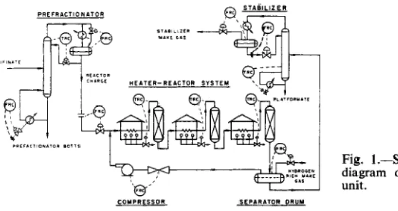
The schematic flow sheet of the process is given in Fig. 1 and simplified block diagram in Fig. 2. The crude feed passes through a prefractionator to remove the heavy ends. The fresh reactor charge plus hydrogen recycle passes through a series of preheater furnaces and catalytic bed reactors.
On leaving the last reactor the crude product is flashed in a separator drum.
Three streams leave the separator; hydrogen-rich gas used for recycle, hydrogen-rich make-gas, and feed for the stabilizer. The bottoms of the stabilizer represent the desired product, the platformate. The stabilizer is usually controlled to produce a certain vapor pressure platformate.
The bead-like platformer catalyst consists of an alumina base which con
tains platinum and chloride-fluoride. It is designed to promote dehydro- genation and acid-isomerization.
The reactions occurring in the catalytic reformer are very complicated
13-60143045 I db Μ
Fig. 1.—Schematic flow diagram of platforming unit.
COMPRESSOR SEPARATOR DRUM
but may be classified as follows: (1) Direct dehydrogenation of 6-membered ring naphthene to aromatics. (2) The isomerization of the 5-membered ring naphthenes to 6-membered ring naphthenes with subsequent dehydrogena- tion to aromatics. (3) The dehydrocyclization of paraffin materials to aro- matics. (4) The hydrocracking of long-chain paraffins. (5) The isomerization of paraffins.
The dehydrogenation and isomerization reactions are rapid and endo- thermic. The hydrocracking reaction is slow and exothermic. A s a conse- quence of this, the temperature drops across the reactors are indicators of how the various reactions are proceeding.
The platformer product is essentially olefin free and has low sensitivity (difference between motor octane number and research octane number).
It contains primarily isoparaffins and aromatics with only a small amount of normal paraffins. The platformate is very low in sulfur and nitrogen.
P R O C E S S A N A L Y S I S
For this discussion here we limit ourselves to the reactor part of the reformer unit. W e assume by this that the prefractionator and the stabilizer can per- form efficiently to handle any product rate and quality that the model of the reactor system requires.
Hydrogen rich make gas ( 1 - k3B ) X5
Stabilizer make gas ( 1 - k4B ) X5
Fresh naphtha feed
x1 x2 x3
Reactor temperatures
x5b Fig. 2.—Simplified block
tformate diagram.
The proper operation of the catalytic reformer requires that the unit produce the required quantity of product at the octane number level which will produce the maximum rate of profit without degrading the catalyst excessively. By experience it is known that the life and efficiency of the catalyst is dependent on the quantity of product produced and the octane level. High octane is obtained at the price of shorter catalyst life. Since the cost of the platinum catalyst is a major item in the operation of the catalytic reformer, it behooves the operator to control his unit carefully. In fact one of the principle areas of payout is the determination of the optimal period for regeneration and/or replacement of the catalyst.
It should be mentioned here that the catalyst is susceptible to poisoning of either temporary or permanent nature. The performance of the catalyst is also function of its past history.
Because the reactors are so complicated the chemical engineer does not attempt to set up a theoretical kinetic rate model. H e rather describes the process in terms of correlations which include the terms which can be manipulated or controlled. These terms may or may not be fundamental in the strict kinetic sense. In particular the chemical engineer evaluates the platformer performance in terms of the product yield in barrels and the product quality in octane number. These are correlated with feed rate, feed characteristics, and reactor inlet operating temperature.
By the previous analysis of the process [2] we may list the independent variables as: Xx = N o . 1 reactor inlet temperature; X2 = N o . 2 reactor inlet temperature; X3 = N o . 3 reactor inlet temperature; X± = Hydrogen mol fraction in reactor charge, =H2 in recycle in mo\s/(X5 + recycle) in mols;
X5 = Reactor charge rate, Bbls/unit time; X6 = Feed A S T M Engler 10 per cent point; X1 = Feed A S T M Engler 90 per cent point; X8 = Naphthene content of feed, vol.%; XQ = Aromatic content of feed in vol.%; X10 = The relative catalyst activity, where X10 varies from 1 for a new catalyst to 0 for a completely spent catalyst.
The term X10 has been evaluated from tests on the catalyst. A general expression for the relative catalyst activity is:
x1 0= i - rl°{ X A X o ) l k a X A 0 )
ki m
where Lt = 2 C^eV W = the cumulative throughput of fresh feed per pound of catalyst. The summation is over the life of the catalyst from the first day (where i = 1) until the catalyst must be replaced or regenerated (where i = m).
W = total weight of the catalyst in the reactors in pounds; AO = base or reference temperature, ° F ; XA = weighted average reactor temperature, °F;
kx and k2 = constants for a particular catalyst.
The term XA is found by summing the product of the average inlet and outlet temperature for each reactor and the relative quantity of catalyst in each reactor.
_ Λ
(Xx + Xe)ji = l £
where Xi = inlet temperature to each reactor (Xl9 X2, X3); Xe = exit tem
perature from each reactor; rx = relative amount of catalyst in the ith reactor.
From the X10 equation we observe that the relative catalyst activity is a function of cumulative throughput of fresh feed and the weighted average reactor temperature. Since the temperature term is an exponential it has a greater effect. The inlet temperatures to each reactor is controlled while the exit temperature is only measured.
Of the independent variables only XS9 X8, X9 cannot be manipulated.
The others can be varied at will over limited ranges.
The correlation equation for the octane yield is written as:
9
θ = a0 +
Σ
a, X% + a10 log X10. (2)The correlation equation for platformate yield is expressed in barrels of platformate/barrel of fresh feed.
B = b0+ ibiXi + b10logX10. (3)
The terms ax and bx are determined from a statistical analyses of the plant data.
A common approach to the catalyst replacement problem, used in refer
ence [2], is to operate the reactor day by day and then ask each day whether it is time to replace the catalyst. This feedback procedure does not predict what values the process variables should take. It does not guarantee that an optimal path is being pursued even though it does calculate the average daily profit.
In contrast to this, it is the approach of this paper to predict the optimal path for the variables to take by dynamic programming. A s a consequence the catalyst replacement policy will also be optimal.
The two yield equations for product yield and product octane are suffi
cient to describe the process. Implied in them are heat balance, material balance, kinetic and thermodynamic equations. These equations also take care of the fact that there are different quantities of catalyst in each bed.
The profitability equation for the platformer when on stream may be written as:
(^ΐ)πιΐη ^ X\ ^ (Xl)max (7) ( ^ O m i n ^ (^5)max (11)
C^2)min ^ X2 ^ (^2)max (8) (12)
(A^min ^ ^ 3 ^ ( ^ 3) m a x (9) < 1 5 ° F (13)
( ^ 4) m l n ^ ^ 4 ^ (^4)max (10) (X3-X2)<15°F (14)
Chimin
(15)D Y N A M I C P R O G R A M M I N G
Dynamic programming embraces the area of multi-stage decision processes.
Through it one can maximize or minimize a function over a number of stages, where the stages may be stages of time or stages in any sequential operation. In particular one desires to make a decision in stage N, so that the consequences of this decision is the best in the light of the (N—l) remaining stages. Bellman [1] expresses this thought in the Principle of Optimality which states that, " A n optimal policy has the property that whatever the initial state and initial decision are, the remaining decisions must constitute an optimal policy with regard to the state resulting from the first decision."
It is necessary to define the state of the system and the transformed state of the system in passing from one stage to another. The state of the system refers to the parameter or parameters which characterize the system. For
Ρ = Β X5 VB + (1 - k3 Β) X, VG + (1 - k, B) X6 VG - X, Vv - V?, (4) Value of Value of the Value of the Variable Fixed
platformer separator stabilizer costs costs product off-gases off-gases
where BX5 = platformer product in barrels/unit time; VB = value of the platformate $/barrel; k3 = constant; (l-k^B), (1 -kzE) = barrels of off gas/unit time; VG = value of off gas $/barrel; Vv = variable cost, $/barrel;
and Vc = fixed cost, $. The value of the platformate product depends on its octane level: VB = Ve 0, where Ve = the value of an octane-barrel.
The equations (2), (3), and (4) are subject to the daily production con
straint that the production of platformate is fixed plus or minus a certain increment.
BX5 = kb±Ak5. (5)
There is also an octane number constraint.
The variables may also be constrained as:
(6)
D E T E R M I N I S T I C C A S E
W e desire to determine for the catalytic reformer the maximum profit-time function, the process variables-time function, and the catalyst replacement and/or regeneration policy.
For the dynamic programming formulation of the deterministic case we assume that all the coefficients in the yield equations (at and b{) are con
stants. W e now define the following terms:
fN(S) = The maximum cumulative profit for an TV-stage process begin
ning in state S and pursuing an optimal policy. TV refers to the number of stages remaining.
7V=1,2,...,JV.
S = X10 = The State of the system characterized for the platformer by relative catalyst activity. It is a function of the cumulative feed rate and the temperature level at which the feed was treated. The state S varies of 1 to 0 where the activity for a fresh catalyst has the value of 1 and a completely spent catalyst the value of zero.
g(S9Xl9 X29 X39 X^9X59X7) = The profit for stage Ν only for the choice of values for Xl9 X29 X& X^ X5, X7 respectively.
h(S) = X10 — ΔX1 0 = The transformed state of the system following the values chosen for Xl9 X29 XZ9 XA9 Χδ9 X7. The term X10 represents the state of the system at the beginning of stage N. The term Δ Ι1 0 is the decremental change in the catalyst activity for the values of the Xt's.
R = The cost of shutting down, regenerating, or replacing the catalyst.
the catalyst replacement problem the state of the system is given by the relative catalyst activity, X10. This term represents the degradation of the catalyst. If there were no degradation, then the state of the system would be invariant and there would be no optimization problem.
In dynamic programming a recursion relationship is developed between the profitability function in stage Ν and stage N—l. A starting point for the determination of the profitability function is the numerical evaluation of the one-stage process. If one knows the profit for a one stage process then by the recursion relationship he can determine the profit for a two- stage process, etc.
The dynamic programming solution in effect starts at the end of the process (with only one stage remaining) and works toward the beginning.
Once an optimal path is found in this manner, it is easy to move forward in time. The question of how one knows beforehand where the process ends may be answered simply by considering a number of possible terminal points and work toward the beginning.
W e may now write the functional relationships for the deterministic case.
[ [g (S, Xl9 X29 XZ9 X4, Xh9 X7) (h (S))l)
MS) = Max\ (16)
Λ OS) = Max [g (S9 Xl9 X29 XZ9 X,9 X59 X7)]9 (17) where the maximization is taken over Xl9 X29 X39 X±9 Χδ9 X7.
The above equations are subject to the constraints equations (5) through (15). Equation (16) states that we must choose the larger of two contending possibilities at each stage of the process. The maximization is done by the proper choice of values for Xl9 X29 XS9 X^9 X59 X7. The equation (16) con
sists of two parts. The first line on the right describes the case of continuing to operate the reactor. The second line describes the possibility of shutting down the reactor, regenerating or replacing the catalyst and beginning over again with a new catalyst.
Referring to the first line of equation (16) the first term describes the profit for stage Ν only. The term g(S9Xl9 X29 X39 X^9 X59 X7) is simply the profit equation (4) evaluated for stage Ν only. The second term fN-i(h(S)) describes the maximum profit over the (N-l) remaining stages beginning in the transformed state h(S). The equation (16) requires this first line to be as large as possible.
In second line of equation (16) the first term R represents the cost for shutting down, regenerating, or replacing the catalyst. The next term/#_ι(1) represents the maximum profit for the (N—\) remaining stages beginning with the catalyst in state one (a fresh catalyst). It is assumed it takes one stage of time for the replacement or regeneration.
The equation (17) describes the one stage process.
D I S C U S S I O N
W e note in this formulation that given N9 the number of stages remaining, and 5, the state of the system, that the maximum profit over the Ν stages remaining is determined. The equation (16) expresses a recursion relation
ship between the profitability in stage Ν and stage (Ν— 1). On passing from stage TV to stage (Ν— 1), the state of the system declines. There is, therefore, a relationship from one state to another in passing from one stage to an
other.
In order to get a solution to this problem, there must be an initial point of departure for the recursion expression. The equation (17) for the one- stage process can be solved and the results of its solution used to develop the profit for the two-stage process.
T A B L E I .
No. of stages / State of the remaining, Ν / system, S
Ν St S2 S3 Si S5 S6
1 f , ( S i ) f , ( S2) f ^ S j ) f , ( S4) f, (S5) MS6) 2 fjfS,) f2(S2> f2( S j ) . ^ « r - ' . 3 f3( S i ) f3( S2) j j J S j ) - -*T
* f4(Si)^MS2)"_MS3) . · ^ — s8 U (s8)
Ν fN( S , ) fN( S2) fN( S3) ' Conti
C O M P U T A T I O N A L A S P E C T S
The dynamic programming formulation requires that certain expressions be maximized. It does not specify how the maximization should be carried out.
The equations (16) and (17) may be solved numerically by a search tech
nique. One method would be to set up a grid of the manipulatable variables and try each combination of variables at each node. While this may seem prohibitive at first, it is not unreasonable in many instances due to the large number of constraints. The constraint equations reduce considerably the feasible region, and many of the possible combinations are ruled out.
The equations (16) and (17) are solved by assuming discrete states of the system and building up a profitability table. In Table I, the heading of the columns are labeled Sl9S2,...9 to indicate arbitrary states. The rows are numbered 1,2,...,TV. Each entry in the table represents fN(S).
The equation (17) is used to develop line 1 of the Table I. For example, for a one stage process beginning in state S = 1, the function Λ( 1 ) is eva
luated by examining all combinations of the Xx terms, consistent with the constraints equations (5) through (15). The largest value is listed a s / i ( l ) . Similarly for each state in a one-stage process, the fx(S)9 the maximum profit is found.
The second line of Table I is developed by using equations (16) and (17).
For example, to find f2(\) requires finding the values of the X{ terms for stage 2 only so that the profit for stage 2 only plus the profit for stage 1 only is a maximum.
The choosing of the Xx terms for stage 2 only transforms the state of the system from S = 1 in stage 2 to S = 1 - ΔΧ10 at the beginning of stage 1.
The maximum profit for stage 1, however, has already been found and is listed in line 1. In essence for each state in stage 2, a search must be made to find the values of Xx terms in stage 2 that cast the system in such a state for the remaining one stage that the overall profit for the two stages is a
maximum. A detailed numerical example is given in reference [3]. Associated with each entry in the Table 1, are the values of the Xx terms that yield the maximum profit. The description of the computational technique is merely a transliteration of the equations (16) and (17).
Having developed this table one can trace the path of optimal operation through it, as shown in Table I. The table shows that, as we move to older and older catalyst for each stage, the profit decreases. The table is also divided into two decision regions. On one side of the line the decision is to always continue operating. On the other side the decision is to shut down for one stage and regenerate the catalyst.
From this table one can determine the number of stages between cata- lyst replacement and/or regeneration and the value of the manipulatable variables at each stage.
S T O C H A S T I C M O D E L
The correlation equations for the product rate and product quality were based on plant data. Due to difference in the efficiency of regeneration, differences in the quality of various batches of catalyst, differences in the relative weight of catalyst use, temporary and permanent catalyst poisoning, channeling, etc., the performance of the catalytic reformer varies. The un- certain nature of these events, the relative and shifting importance of one with respect to the others causes us to look up to the process as a stochas- tic one.
In particular, in the stochastic model of the catalytic reformer, the co- efficients of the Xx terms must be considered as probabilistic terms. W e assume here that the shape of the yield equations hold for both the deter- ministic and stochastic models.
The problem that we seek to solve therefore is to optimize the profitability of the reactor over a number of stages, to determine the variables-time function, and the catalyst replacement or regeneration policy in the face of this uncertainty.
W e take here a self-adaptive approach to the problem. W e claim that the past history of the process can be used to regenerate the coefficients in the yield equations. With the most up-to-date coefficients available, then the yield equations can be used as predictors.
In an earlier paper two general classes of stochastic cases were consi- dered; those in which the probability distribution of the ax and bx terms were known and those in which the distributions were unknown.
Let us consider here only the first case. W e therefore can define the ex- pected value of the ax terms as
oo
E(at) = j a,ρ (a,)da,, (18)
-oo
where E(at) = the expected value of a{\ p(a^) = the probability distribution of the a{ terms. Similar expressions define
The correlation expressions for the product yield and the octane yield now can be defined as the expected product yield and the expected octane yield.
In view of the stochastic nature of the process it is not possible to define the profit in terms of maximum profit as described for the deterministic case. W e must compromise and the best we can do is to define the profit in terms of an expected maximum profit.
The following terms may now be defined:
FN(S) = The expected maximum profit for an Ν stage process beginning in state S and pursuing an optimal policy.
S = The state of the system defined by X10.
G [S, Xl9 X29 XZ9 X,9 Xb9 Xl9 E(a0)9 E(ax)9..., E(a10)9 E(b0)9 E(bx)9 E(b10)]
= The expected profit for stage Ν for the choice of values for Xl9 X29
XS9 X±9 X59 X7 where E(a^) and E(bi) are the expected values for the coeffi
cients.
h(S) = T h e transformed state of the system.
R = The cost of shutting down, regenerating or replacing the catalyst.
The expected maximum profit equation may be formulated as:
FN(S) = Mzx
F±(S) = Max
Max {G[S9X19X29XZ9 X,9 X59 X79 E(a,)9E(ax)9 ...,£«), E(b0)9 E(bx)9..., E(b10)] + (h ( 5 ) ) } ;
-R + FN^(l)
G[S9X19 E(a0),E(a1),...,E(a10),}
E(b0),E(b1),...,E(b10)] j
(19)
(20) where the maximization is taken over Xj_9 X2i X& X& X& Χη>
The meaning of these equations is clearly parallel to the discussion for the deterministic case.
While it appears at first that the stochastic case is much more cumber
some and involved than the deterministic case, in actuality it is not so unwieldy.
T o evaluate the equations we recognize the fact that during any given stage that measurements and sample analyses may be taken on the process.
A s a consequence of this some (or perhaps all) of the coefficients may be evaluated for that particular stage. The measured value of each coefficient is pooled with previous values of the coefficient to give an up-to-date estimate of the coefficient value. This self-adaptive feature makes it possible
for the model to represent the process more truly. The pooled estimates of the coefficients are then used for prediction.
The method of pooling the data to represent the coefficients depends on the process itself. The coefficients may be found by simple arithmetic averaging. The coefficients may be found by weighting the most recent data heavier than the earlier data. A study of the past data of the process should reveal whether and how the mean and/or the standard deviation for each coefficient moves with time.
The sequence of events goes something like this. A t the beginning of the Ν stage process, that is at stage N, some estimates of the coefficients are known. Using these coefficients the equations and the profitability table are evaluated for the remaining Ν stages. During stage Ν measurements and analyses are taken to evaluate the coefficients. A pooled estimate of the a priori estimates with the recently determined estimates of the coefficients is formed. With the newly pooled estimates of the coefficients in the equa
tions (19) and (20), the profitability table is generated once again for the (N-\) remaining stages. This procedure is carried out over and over again as more information is developed.
For all practical purposes the stochastic model reduces to the determinis
tic case because the estimates of the coefficients are considered to be con
stants over the remaining number of stages. The stochastic model differs from the deterministic model in that the equations (19) and (20) and the profitability table must be evaluated over and over again as new infor
mation about the coefficients is gathered.
D I S C U S S I O N
In catalytic reforming "blocked" operations are often used. That is, quan
tities of similar feed stock are processed for perhaps five days continuously and then another type of feed stock is processed for perhaps four days, etc.
The practical aspect of reformer operation can be handled very neatly by dynamic programming for both the deterministic and the stochastic cases. Depending on how different the feed stocks are, the yield equations may describe the behavior of both feeds, or the coefficients may differ from one feed to another, or the shape of the yield equations may differ.
For any of these possibilities the methodology of dynamic programming is equally facile.
Another area where dynamic programming can be useful is to determine for "blocked" operation what is the best sequence and the duration of processing each feed stock. This will require that the refinery specify what sequence and duration are feasible in a practical sense. By solving the
C O N C L U S I O N
W e have discussed the importance and general process features of catalytic reforming. The process is characterized by yield correlations for the product rate and for octane number. By dynamic programming methods the catalyst replacement problem may be formulated and solved. The solution yields the maximum profit-time function, the octane-time function, the process variables-time function, and the catalyst replacement or regeneration policy.
Due to uncertainties in catalyst regeneration, channeling, catalyst quality, temporary or permanent poisoning, catalytic reforming may be considered a stochastic process, where the probabilistic elements are associated with the coefficients of the yield equations. If the process is considered as a self adaptive (self-learning) process, then the stochastic formulation of the dynamic programming problem reduces essentially to the deterministic case.
R E F E R E N C E S
1. BELLMAN, R., Dynamic Programming. Princeton University Press, 1957.
2. LANE, J. W., Digital Computer Control of a Catalytic Reforming Unit. Instrument Society of America Conference, Houston, February 1-4, 1960, Preprint 17-H60.
3. ROBERTS, S. M., The Dynamic Programming Formulation of the Catalyst Replace
ment Problem. CEP Symposium Series 56, no. 31, 103-110 (1960).
4. ROBERTS, S. M., Stochastic Models for the Dynamic Programming Formulation of the Catalyst Replacement Problem. Proceedings of the Optimization Techniques in Chemical Engineering Symposium sponsored by New York University, AIChE, ORSA, May 18, 1960.
5. SMITH, R. B . and DREPER, ΤΗ., Petrol. Refiner 36, no. 1, 199-202 (1957).
catalyst replacement problem sufficient number of times to cover the practical scheduling possibilities for the "blocked" operation, an optimal
"blocked" operation can be found.