A Brief Survey and Comparison on Various Interpolation Based Fuzzy Reasoning Methods

A Brief Survey and Comparison on Various Interpolation Based Fuzzy Reasoning Methods

Zsolt Csaba Johanyák

, Szilveszter Kovács

1 Department of Information Technology, GAMF Faculty, Kecskemét College, H-6001 Kecskemét, Pf. 91, johanyak.csaba@gamf.kefo.hu

2 Department of Information Technology, University of Miskolc, Miskolc- Egyetemváros, H-3515 Miskolc, Hungary, szkovacs@iit.uni-miskolc.hu

Abstract: Fuzzy systems based on sparse rule bases produce the conclusion through approximation. This paper is the first part of a longer survey that aims to provide a qualitative view through the presentation of the basic ideas and characteristics of some methods and defining a general condition set brought together from an application- oriented point of view.

Keywords: interpolative fuzzy reasoning, sparse rule base

1 Why do We Need Interpolation?

The functioning of systems working with fuzzy logic is based on rules. The rule base is considered dense when for all the possible observations there exists at least one rule, whose antecedent part overlaps the input data, at least partially.

Otherwise, the rule base is considered to be sparse. The classical inference methods (e.g. compositional rule of inference) are not able to produce an output for the observations covered by none of the rules. That is why the systems based on a sparse rule base should adopt inference techniques, which in the lack of matching rules perform an approximate reasoning taking into consideration the existing rules. The most often used methods for this purpose are called interpolative methods.

2 General Conditions on Rule Interpolation Methods

A unified condition system related to the interpolative methods would make the evaluation and comparison of the different techniques based on the same

fundamentals possible. However, according to the existing literature (e.g. [1] [6]

[16] [18]) can be found only partly consistent conditions and condition groups, which are put together taking different points of view into consideration.

Therefore, as a step towards the unification, the conditions considered to be the most relevant ones from the application-oriented aspects are going to be reviewed and based on them, some of the well known methods are going to be compared in the followings.

General conditions on rule interpolation methods:

1 Avoidance of the abnormal conclusion [1] [6] [16]. The estimated fuzzy set should be a valid one. This requisite can be described by the constraints (1) and (2) according to [16].

{ } sup { } [ ] 0 , 1

inf B

≤ B

∀ α ∈

{ } inf { } sup { } sup { } [ ] 0 , 1 inf B

≤ B

≤ B

≤ B

∀ α

< α

∈

^inf { } B

^sup { } B

2 The continuity of the mapping between the antecedent and consequent fuzzy sets [1] [6]. This condition indicates that similar observations should lead to similar results.

3 Preserving the “in between” [6]. If the antecedent sets of two neighbouring rules surround an observation, the approximated conclusion should be surrounded by the consequent sets of those rules, too.

4 Compatibility with the rule base [1] [6]. This means the requisite on the validity of the modus ponent, namely if an observation coincides with the antecedent part of a rule, the conclusion produced by the method should correspond to the consequent part of that rule.

5 The fuzziness of the approximated result. There are two opposite approaches in the literature related to this topic [18]. According to the first subcondition (5a), the less uncertain the observation is the less fuzziness should have the approximated consequent [1] [6]. With other words in case of a singleton type observation the method should produce a crisp valued consequence. The second approach (5b) originates the fuzziness of the estimated consequent from the nature of the fuzzy rule base [16]. Thus, crisp conclusion can be expected only if all the consequents of the rules taken into consideration during the interpolation are singleton shaped, i.e. the knowledge base produces certain information from fuzzy input data.

6 Approximation capability (stability [e.g. 17]). The estimated rule should approximate with the possible highest degree the relation between the

antecedent and consequent universes. If the number of the measurement (knot) points tends to infinite, the result should converge to the approximated function independently from the position of the knot points.

7 Conserving the piece-wise linearity [1]. If the fuzzy sets of the rules taken into consideration are piece-wise linear, the approximated sets should conserve this feature.

8 Applicability in case of multidimensional antecedent universe.

9 Applicability without any constraint regarding to the shape of the fuzzy sets.

This condition can be lightened practically to the case of polygons, since piece-wise linear sets are most frequently encountered in the applications.

3 Surveying Some Interpolative Methods

The techniques being reviewed can be divided into two groups relating to their conception. The members of the first group produce the approximated conclusion from the observation directly. The second group contains methods that reach the target in two steps. In the first step they interpolate a new rule whose antecedent part overlaps the observation at least partially. The estimated conclusion is determined in the second step based on the similarity between the observation and the antecedent part of the new rule.

Further on mostly the case of the one-dimensional antecedent universes are presented for the sake of easy understanding of the key ideas of the methods. As several methods need the existence of two or more rules flanking the observation, therefore it is assumed that they exist and are known. The methods are not based on the same principles, hence sometimes they approach the topic of the rule interpolation from different viewpoints.

3.1 The Linear Interpolation Introduced by Kóczy and Hirota and the Derived Methods

The first subset of the methods producing the approximated conclusion from the observation directly contains the technique introduced by Kóczy and Hirota and those ones that have been derived from it aiming its extension and improvement.

First the most famous member of this group, the KH interpolation is reviewed.

3.1.1 KH Interpolation

The key idea of the method developed by Kóczy and Hirota [8] is that the approximated conclusion divides the distance between the consequent sets of the

used rules in the same proportion as the observation does the distance between the antecedents of those rules (3). This is the fundamental equation of the fuzzy rule interpolation [1]. The proportions are set up separately for the lower and upper distances in the case of each α-cut.

The development of KH method was made possible by the definition of the fuzzy distance [7] and the fact that the fuzzy sets can be decomposed into α-cuts and can be composed from α-cuts (resolution and extension principle).

( ) ( ) (

) (

)

1 2

*

*

1

, A : d A , A d B , B : d B , B

A

d

=

where A1, A2 are the antecedent sets of the two flanking rules, A^* is the observation, B1, B2 are the consequent sets of those rules, B^* is the approximated conclusion, i can be L or U depending on lower or upper type of the distance. The technique adopted for the determination of the consequent is an extension of the classic Shepard interpolation [12] for case of the fuzzy sets. The method requires the following preconditions to be fulfilled: the sets have to be convex and normal with bounded support, and at least a partial ordering should exist between the elements of the universes of discourses. The latter one is needed for the definition of the fuzzy distance.

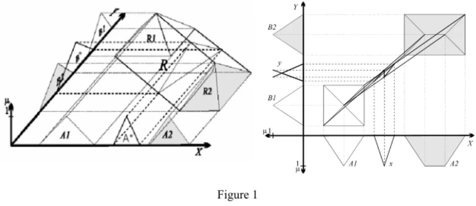
The most important advantage of the KH interpolation is its low computational complexity that ensures the fastness required by real time applications. Its detailed analysis e.g. [10] [9] [13] led to the conclusion that the result can not be interpreted always as a fuzzy set, because e.g. by some α-cuts of the estimated consequent the lower value can be higher than the upper one (Fig. 1). The above listed publications defined application conditions that enabled the avoidance of the abnormal conclusion.

Figure 1 KH interpolation

Theoretically, an infinite number of α-cuts are needed for the exact result if there are no conditions related to the shape of the sets. However, in practice driven by need for efficiency mostly piece-wise linear generally triangle shaped or trapezoidal sets can be found, because these can be easily described by a few

characteristic points. Thus supposing the method preserves the linearity completing the calculations for a finite small number of α-cuts could be enough.

Although the preceding assumption is not fulfilled, in most of the applications it does not matter because of the negligible amount of the deviation [10] [9] [16].

The KH method was developed for one-dimensional antecedent universes.

However, it can be applied in multi-dimensional case using distances calculated in Minkowski sense. It can be simply proven that this technique fulfils conditions 3, 4, 5b and 8. The stabilized (general) KH interpolation [17] also satisfies the condition 6.

The recognition of the shortcomings of the KH interpolation has led to the development of many techniques, which modified or improved the original one or offered a solution for the task of the interpolation using very new approaches.

Further on some methods improving the KH technique are reviewed emphasizing those properties which are considered to be the most important.

3.1.2 Extended KH Interpolation

Several versions of the KH interpolations were developed which allow taking into consideration more than two rules during the determination of the consequence.

Their common feature is that the approximation capability of the technique is getting better with the growth of the number of the rules taken into consideration.

In [8] a technique is proposed that takes into consideration the rules weighted with e.g. the reciprocal value of the square of the distance. This approach reflects that the rules situated far away from the observation are not as important as those ones in the neighbourhood of the observation.

The authors of [17] suggest to use formulas for the calculation of endpoints of α- cuts of the approximated consequence, which contain the distance on the n^th power, where n is number of the antecedent dimensions.

3.1.3 The VKK Method

Figure 2

The method developed by Vass, Kalmár and Kóczy [19] worked out the problem of abnormal conclusion introducing modified distance measures (Fig. 2). The method is an α-cut based technique. It describes each α-cut by the position of its centre point and its width (w). The distance of the sets is characterized by a vector containing the Euclidean distances of the centre points (d). The method is also applicable in multidimensional case by calculating the resulting distance in Minkowski sense with the parameter 2 and by determining the resulting width as a geometric mean of the width values in each dimension. However, the technique cannot be applied if any of the antecedent sets taken into consideration during the interpolation are singleton shaped (none of the antecedent α-cut widths can be zero valued). Like the KH method it does not conserve the linearity, but the deviance can be proven to be negligible [1].

It can be simply proven that this technique fulfils conditions 3, 4, 5.a and 8.

3.1.4 Modified α-cut Based Interpolation

The modified α-cut based interpolation (MACI) [16] represents each fuzzy set by two vectors describing the left (lower) and right (upper) flanks using the technique published by Yam [21]. The vectors contain the break points in case of piece-wise linear membership functions or endpoints of predefined (usually uniform distributed) α-cuts in case of smooth membership functions. For example the antecedent set A1 in Fig. 3 is represented by the vectors (4) and (5).

[

]

1

1

x , x

A

=

[ ]

1

x , x

A

=

Figure 3

The graphical representation of the vectors describing the right flanks of the sets can be seen on the Figure 4. The antecedent and consequent sets are represented separately. The result will fulfil the condition 1 if B* is situated inside of the rectangle and above of the line l. This purpose is reached through a coordinate transformation where Z0 is substituted by the line l. The approximated conclusion

will be crisp only if the consequent sets of the rules taken into consideration are singletons, as well.

Although this method is not conserving the linearity, the deviance is smaller than in the case of the KH interpolation [16] and the stability experienced at the KH method [15] remains. The estimated conclusion always yields fuzziness if the consequent sets of the rules taken into consideration have fuzziness [22].

Figure 4

Graphical representation of the vectors [18]

It can be proven that the technique fulfils the conditions 1-4, 5b, 6, 8 and 9 with the constraint that the sets should be convex and normal. Its generalized version [14] can be used in case of non-convex fuzzy sets, too.

3.1.5 The Improved Multidimensional Modified α-cut Based Interpolation The improved multidimensional modified α-cut based interpolation (IMUL) introduced by Wong, Gedeon and Tikk [20] combines the advantages of the MACI and the fuzziness conservation technique proposed by Kóczy and Gedeon in [3]. This method was developed for the case of multidimensional antecedent universe. The fuzzy sets are described by vectors containing the characteristic points, and the coordinate transformation introduced by MACI is used during the determination of the core of the approximated consequent.

Figure 5 [23]

The fuzziness of the observation (r) plays a decisive role at the calculation of the flanking edges and beside this the relative fuzziness of the sets adjacent to the observation (s/u) and adjacent to the approximated consequent (s’/u’) are taken into consideration, as well. Figure 5 presents the meaning of the used notation for the case of the right flank of the conclusion.

It can be proven that the technique fulfils the conditions 1-4, 5a, 6, 8 and 9 with the constraint that the sets should be convex and normal.

3.2 Fuzzy Rule Interpolation in the Vague Environment

The fuzzy rule interpolation in the vague environment (FIVE) introduced by Kovács [11] puts the problem of rule interpolation in a virtual space in the so- called vague environment whose conception is based on the similarity (indistinguishability) of the objects. The similarity of two fuzzy sets in the vague environment (6) is characterized by their distance weighted with the so-called scaling function (s), which describes the vague environment. The scaling function describes the shapes of all the terms in a fuzzy partition.

( ) ⁼ ∫

( )

dx x s ,

1

x s

x x

δ

Figure 6

The challenge during the employment of this method is to find approximate scaling functions for both the antecedent and the consequent universes, which give good descriptions in case of non-Ruspini partitions, too. Scaling functions for the case of triangle and trapezoid shaped fuzzy sets are given in [11]. In consequence of the creation of the vague environments of the antecedent and consequent universes, the vague environment of the rule base is established, as well. In this environment each rule is represented by a point. If the observation is a crisp set, the conclusion, which will be crisp, can be also determined employing any interpolative or approximate technique.

The possibility of creation of the antecedent and consequent vague environments in advance ensures the fastness and hereby the applicability of the method for real-

time tasks. Thus, only the interpolation of the points describing the rule base has to be made during the functioning of the system. In case of fuzzy observations the antecedent environment should be created taking into consideration the shape of the set, which describes the input.

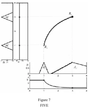
Figure 7 presents the partitions, the scaling function and the curve built from the points defined by the existent two rules and the points interpolated for the case of a one dimensional antecedent universe supposing crisp observations. The method satisfies the conditions 1-4, 5a, 6 and 8.

Figure 7 FIVE

3.3 The Generalized Methodology

Baranyi, Kóczy and Gedeon proposed in [1] a generalized methodology for the task of the fuzzy rule interpolation. In the centre of the methodology stands the interpolation of the fuzzy relation. A reference point, which can be identical with e.g. the centre point of the core, is used for the characterization of the position of fuzzy sets. The distance of fuzzy sets is expressed by the distance of their reference points. The interpolation is broken down to two steps.

In the first step an interpolated rule is produced, whose antecedent has at least a partial overlapping with the observation and whose reference point coincides with the reference point of the observation. This task is divided into three stages. First with the help of a set interpolation technique the antecedent of the new rule is produced. Next the reference point of the conclusion is interpolated going out

from the position of the reference points of the observation and the reference points of the sets involved in the rules taken into consideration. The applied technique can be a non-linear one, too. Hereupon the consequent set is determined similarly to the antecedent one. Several techniques are suggested in [1] for the task of set interpolation (e.g. SCM, FPL, FVL, IS-I, IS-II). In this paper the solid cutting method is presented in section 3.3.1. If λa (Fig. 8) denotes the ratio, in which the reference point of the observation divides the distance between the reference points of the neighbouring sets into two parts and λc denotes the similar ratio on the consequent side, the function λc=f(λa) defines the position of the reference point of the consequent set. Through the selection of the function f() a whole family of linear (λc=λa) and non-linear interpolation techniques can be derived. This is also a possibility for parameterisation (tuning) of the methodology, which ensures the adaptation to the nature of the modelled system.

The approximated rule is considered as part of the rule base in the second step.

The conclusion corresponding to the observation is produced by the help of this rule. As the antecedent of the estimated rule generally does not fit perfectly to the observation, some kind of special single rule reasoning is needed. For example the similarity transfer method introduced in [13], the revision principle based FPL and SRM techniques presented in [24] or the scale and move transformations based method [5] can be applied with success in this step. As a precondition for the revision principle based methods, it should be mentioned that the support of the antecedent set has to coincide with the support of the observation. Generally this is not fulfilled. In such cases the fuzzy relation (rule) obtained in the previous step is transformed first, in order to meet this condition.

Owing to the modular structure of the methodology in both of the steps one can choose from many potential methods if some conventional elements (e.g. distance measure) are used consequently. Based on the analysis in [1] and [22] the methodology can be characterized as follows. Conditions 1-4, 5a and 8 are satisfied applying any of the suggested methods in [1]. In case of triangle shaped fuzzy sets the condition 7 is also fulfilled by those techniques. Condition 9 is also satisfied if SCM or FPL is used in the first step and FPL is used in the second step.

3.3.1 The Solid Cutting Method

The key idea of the solid cutting method (SCM) [2] developed by Baranyi et al. is to define vertical axes at the reference points of the two antecedent sets (A1 and A2) which flank the observation (A*) and after that to rotate these sets by 90º around the vertical axes. The virtual space created in such mode is determined by the orthogonal coordinate axes S, X and μ. The rotated sets will be situated in parallel plane to the plane μxS (Fig. 8).

In the next step a solid is generated fitting a surface on the contour and support of the sets. After this the solid is cut by the reference point of the observation with a plane parallel with μxS. Turning back the cross section by 90º one will obtain the

antecedent set of the estimated rule. The consequence of the new rule is determined similarly by knowing the two consequent sets and the reference point.

Figure 8 SCM [2]

3.3.2 Single Rule Reasoning Based on Semantic Revision

The antecedent set (Aⁱ) of the interpolated rule generally does not fit perfectly to the observation (A*), therefore some kinds of special single rule reasoning techniques (SRRT) are needed in the second step. Further on the key ideas of the semantic revision based methods are reviewed.

Figure 9

The SRM was introduced by Shen, Ding and Mukaidono [24]. It relies on the concept of the interrelation and semantic relation functions. The interrelation function (IR) is a mapping between the elements of two fuzzy sets. It defines which points of the sets are related to each other (Fig. 9 first quarter). The semantic relation function (SR) is a mapping between the membership values of the interrelated points of two fuzzy sets (Fig. 9 third quarter). In the Fig. 9 there are two semantic relation functions describing the relation between the left flanks and between the right flanks separately.

As a precondition of the application of the SRM it should be mentioned that the support of the antecedent set has to coincide with the support of the observation and the heights of the rule antecedent and the observation A* have to be the same.

In order to fulfil the conditions generally two transformations of the interpolated fuzzy relation (rule) are necessary. First the technique called Transformation of the Fuzzy Relation (TFR) [1] transforms (stretches or shrinks) the interrelation area proportionally by the help of set transformations in order to ensure the needed coincidence of the supports. Secondly the algorithm called Transformation of the Semantic Relation [1] modifies the semantic relation area corresponding to the height of A*.

The SRM methods go out from the transformed sets A^st, B^st and the transformed relation areas (Fig. 9). Its key idea is the assumption that between A* and B* there exists the same interrelation and semantic relation as between A^st and B^st. It means that substituting A^st by A* and abandoning B^st the approximated conclusion can be determined using the existing interrelation and semantic relation. Thus going out from the point yi that belongs to the left edge of B* its membership value can be determined following the dashed lines in the directions given by the arrows.

3.4 Interpolation with Generalized Representative Values

The IGRV method proposed by Huang and Shen [5] follows an approach similar to the generalized methodology. In the first phase, a representative value (RV) is determined for each used set. Its function is the same as the function of the reference point in the generalized methodology. It can be calculated by different formulas depending on the demands of the application. The centre of gravity played this role in the first variant of the method [4], which was developed for triangle shaped fuzzy sets. In case of an arbitrary polygonal fuzzy set the weighted average of the x coordinates of the node (break) points is suggested as RV.

Figure 10

Scale and move transformations [5]

The definition mode of the representative value influences only the position of the estimated rule, but not the shape of the sets involved in the rule. Further on the Euclidean distance of the RVs of the sets are considered as the distance of the sets.

The antecedent of the approximated rule is determined by its α-cuts in such way that two conditions have to be satisfied. First its representative value has to coincide with the RV of the observation. Secondly the endpoints of the α-cuts of the observation have to divide the distance of the respective (left or right) endpoints of the α-cuts of the neighbouring sets in such proportion as the RV of the observation divides the distance of the RVs of these sets. Following the same proportionality principle the representative value and the shape of the consequent of the approximated rule are determined.

In the second phase, the similarity of the observation and the antecedent part of the new rule is characterized by the scale and move transformations needed to transform the antecedent set into the observation. The method was developed primordially for the case of polygonal shaped fuzzy sets. It is applicable in the case of multidimensional antecedent universes, too. In terms of classification, it can be considered as an α-cut based technique, because the scale and move transformation ratios are calculated for each level corresponding to node (break) points of the shape of sets.

The method is well applicable in case of polygonal shaped sets, but the checking and constraint applications done at each α-level for the sake of the conservation of convexity increase the computational complexity of the technique.

It can be tuned at two points. First one can choose the formula for the representative value. Secondly one can choose the method for the calculation of the resulting transformation ratios in the case of multidimensional antecedent universes. On the grounds of the analysis in [5] it can be stated that the method satisfies the conditions 1, 2, 3, 4, 5a, 8, and 9.

Conclusions

Systems working with a conventional inference method in case of a sparse rule base cannot produce a result for all the possible input universe values. In such cases the system should adopt an approximate reasoning technique for the estimation of the conclusion. The surveyed methods can be classified into two fundamental groups depending on whether they are producing the result in one or two steps.

In the first part of this paper a general condition set was brought together containing the features, which can be expected from interpolative methods considering an application-oriented viewpoint. After this some well-known methods were surveyed emphasizing their basic ideas, significant characteristics and the conditions they are fulfilling.

References

[1] Baranyi, P., Kóczy, L. T. and Gedeon, T. D.: A Generalized Concept for Fuzzy Rule Interpolation. In IEEE Transaction On Fuzzy Systems, ISSN 1063-6706, Vol. 12, No. 6, 2004, pp. 820-837

[2] Baranyi, P., Kóczy, L. T.: A General and Specialised Solid Cutting Method for Fuzzy Rule Interpolation, In J. BUSEFAL, URA-CNRS, Vol. 66, Toulouse, France, 1996, pp. 13-22

[3] Gedeon, T. D., Kóczy, L. T.: Conservation of fuzziness in the rule interpolation, Intelligent Technologies, International Symposium on New Trends in Control of Large Scale Systems, Vol. 1, Herlany, 1996, pp. 13- 19

[4] Huang, Z. H., Shen, Q.: A New Interpolative Reasoning Method Based on Center of Gravity, in Proceedings of the 12^th International Conference on Fuzzy Systems, Vol. 1, pp. 25-30, 2003

[5] Huang, Z., Shen, Q: Fuzzy interpolation with generalized representative values, in Proceedings of the UK Workshop on Computational Intelligence, pp. 161-171, 2004

[6] Jenei, S.: Interpolation and Extrapolation of Fuzzy Quantities revisited - (I), An Axiomatic Approach, Soft Computing, ISSN: 1432-7643, 5 (2001), pp. 179-193

[7] Kóczy, L. T., Hirota, K.: Ordering, distance and closeness of fuzzy sets, Fuzzy Sets and Syst., Vol. 59, 1993, pp. 281-293

[8] Kóczy, L. T., Hirota, K.: Rule interpolation by α-level sets in fuzzy approximate reasoning, In J. BUSEFAL, Automne, URA-CNRS, Vol. 46, Toulouse, France, 1991, pp. 115-123

[9] Kóczy, L. T., Kovács, Sz.: Shape of the fuzzy conclusion generated by linear interpolation in trapezoidal fuzzy rule bases, in Proc. 2^nd Eur. Congr.

Intelligent Techniques and Soft Computing, Aachen, Germany, 1994, pp.

1666-1670

[10] Kóczy, L. T., Kovács, Sz.: The convexity and piecewise linearity of the fuzzy conclusion generated by linear fuzzy rule interpolation, In J.

BUSEFAL 60, Automne, URA-CNRS. Toulouse, France, Univ. Paul Sabatier, 1994, pp. 23-29

[11] Kovács, Sz., Kóczy, L. T.: Application of an approximate fuzzy logic controller in an AGV steering system, path tracking and collision avoidance strategy, Fuzzy Set Theory and Applications, Tatra Mountains Mathematical Publications, Mathematical Institute Slovak Academy of Sciences, Vol. 16, pp. 456-467, Bratislava, Slovakia, (1999)

[12] Shepard, D.: A two dimensional interpolation function for irregularly spaced data, Proc. 23^rd ACM Internat. Conf., (1968) 517-524

[13] Shi, Y., Mizumoto, M., Wu, Z. Q.: Reasoning conditions on Kóczy’s interpolative reasoning method in sparse fuzzy rule bases, Fuzzy Sets Syst., Vol. 75, pp. 63-71, 1995

[14] Tikk, D., Baranyi, P., Gedeon, T. D., Muresan, L.: Generalization of the Rule Interpolation method Resulting Always in Acceptable Conclusion, Bratislava, Slovakia, Tatra Mountains, Math. Inst. Slovak Acad. Sci., 2001, Vol. 21, pp. 73-91

[15] Tikk, D., Baranyi, P., Yam, Y., Kóczy, L. T.: Stability of a new interpolation method, in Proc. IEEE Conf. Syst. Man. and Cybern. (SMC

’99), Tokyo, Japan, 1999, pp. III/7-III/9

[16] Tikk, D., Baranyi, P.: Comprehensive analysis of a new fuzzy rule interpolation method, IEEE Trans Fuzzy Syst., Vol. 8, June 2000, pp. 281- 296

[17] Tikk, D., Joó, I., Kóczy, L. T., Várlaki, P., Moser, B., Gedeon, T. D.:

Stability of interpolative fuzzy KH-controllers. Fuzzy Sets and Systems, 125(1) pp. 105-119, January 2002

[18] Tikk, D.: Investigation of fuzzy rule interpolation techniques and the universal approximation property of fuzzy controllers, Ph. D. dissertation, TU Budapest, Budapest, 1999

[19] Vass, Gy., Kalmár, L., Kóczy, L. T.: Extension of the fuzzy rule interpolation method, in Proc. Int. Conf. Fuzzy Sets Theory Applications (FSTA ’92), Liptovsky M., Czechoslovakia, 1992, pp. 1-6

[20] Wong, K. W., Gedeon, T. D., Tikk, D.: An improved multidimensional α- cut based fuzzy interpolation technique, in Proc. Int. Conf Artificial Intelligence in Science and Technology (AISAT’2000), Hobart, Australia, 2000, pp. 29-32

[21] Yam, Y., Kóczy, L. T.: Representing membership functions as points in high dimensional spaces for fuzzy interpolation and extrapolation.

Technical Report CUHK-MAE-97-03, Dept. Mech. Automat. Eng., The Chinese Univ. Hong Kong, Hong Kong, 1997

[22] Mizik, S.: Fuzzy Rule Interpolation Techniques in Comparison, MFT Periodika 2001-04, Hungarian Society of IFSA, Hungary, 2001, http://www.mft.hu

[23] Wong, K. W., Tikk, D., Gedeon, T., Kóczy, L. T.: Fuzzy Rule Interpolation for Multidimensional Input Spaces With Applications: A Case Study, IEEE Transactions On Fuzzy Systems Vol. 13, No. 6, Dec. 2005, pp. 809-819 [24] Shen, Z., Ding, L., Mukaidono, M.: Methods of revision principle, in Proc.

5^th IFSA World Congr., 1993, pp. 246-249