Lebesgue constants in polynomial interpolation

(2006) pp. 109–123

http://www.ektf.hu/tanszek/matematika/ami

Lebesgue constants in polynomial interpolation

Simon J. Smith

La Trobe University, Bendigo, Australia e-mail: s.smith@latrobe.edu.au

Submitted 15 September 2005; Accepted 2 June 2006

Abstract

Lagrange interpolation is a classical method for approximating a contin- uous function by a polynomial that agrees with the function at a number of chosen points (the “nodes”). However, the accuracy of the approximation is greatly influenced by the location of these nodes. Now, a useful way to measure a given set of nodes to determine whether its Lagrange polynomials are likely to provide good approximations is by means of the Lebesgue con- stant. In this paper a brief survey of methods and results for the calculation of Lebesgue constants for some particular node systems is presented. These ideas are then discussed in the context of Hermite–Fejér interpolation and a weighted interpolation method where the nodes are zeros of Chebyshev poly- nomials of the second kind.

Keywords: interpolation, Lagrange interpolation, Hermite–Fejér interpola- tion, Lebesgue constant, Lebesgue function

MSC:41-02, 41A05, 41A10

1. Introduction

For each integern>1, considernpoints (nodes)xk,n(k= 1,2, . . . , n) in[−1,1]

with

−16xn,n < xn−1,n< . . . < x2,n< x1,n61, (1.1) and letX be the infinite triangular matrix

X ={xk,n:k= 1,2, . . . , n; n= 1,2,3, . . .}. (1.2) 109

Givenf ∈C[−1,1], the classical Lagrange interpolation polynomialLn−1(X, f)of degreen−1(or less) for f, based onX, can be written as

Ln−1(X, f)(x) = Xn

i=1

f(xi,n)ℓi,n(X, x),

where the fundamental polynomial ℓi,n(X, x) is the unique polynomial of degree n−1withℓi,n(X, xk,n) =δi,k,16k6n. (Hereδi,k denotes the Kronecker delta.)

Letkfkdenote the uniform norm kfk= max

−16x61|f(x)|.

When studying the uniform convergence behaviour of the Ln−1(X, f)as n→ ∞, a crucial role is played by theLebesgue function

λn(X, x) = max

kfk61|Ln−1(X, f)(x)|= Xn

i=1

|ℓi,n(X, x)|

and theLebesgue constant Λn(X) = max

kfk61kLn−1(X, f)k= max

−16x61λn(X, x) (see, for example, Rivlin [13, Chapter 4] or Szabados and Vértesi [19]).

Now, it is known that forany X, Λn(X) is unbounded with respect to n. A consequence of this is (by the uniform boundedness theorem) Faber’s 1914 result [6]

that there existsf ∈C[−1,1]such thatLn(X, f)doesnotconverge uniformly tof. However, iff is not too badly behaved (as measured by the modulus of continuity, for instance) and theΛn(X)are not too large, then uniform convergenceisachieved (see, for example, Rivlin [13, Chapter 4]).

Figure 1 illustrates some basic properties of Lebesgue functions for Lagrange interpolation. For example, for anyX and n>3,λn(X, x)is a piecewise polyno- mial that satisfies λn(X, x)>1 with equality if and only ifx is one of the nodes xk,n. As well, on each interval (xk+1,n, xk,n) for 1 6 k 6 n−1, λn(X, x) has precisely one local maximum, whileλn(X, x)is decreasing and concave upward on (−1, xn,n) and is increasing and concave upward on(x1,n,1). (For a discussion of these and other properties see, for example, Luttmann and Rivlin [11].)

2. The Lebesgue function for specific node systems

For some particular node systems, the Lebesgue function and constant have been studied in considerable detail. In this section, a summary of some of these results is given — for a more detailed account of many of the results, see the comprehensive survey paper by Brutman [4] and the references therein.

0 1 5 10

–1 1

Figure 1: Lebesgue function for Lagrange interpolation based on the six nodes−0.9,−0.8, 0.1, 0.5, 0.65 and 0.95.

2.1. Equally-spaced nodes

Figure 2 illustrates a typical Lebesgue function for Lagrange interpolation based on the equally-spaced nodes

E={xk,n= 1−2(k−1)/(n−1) :k= 1,2, . . . , n; n= 1,2,3, . . .}. As suggested by the graph, the local maxima ofλn(E, x)are strictly decreasing from the outside towards the middle of the interval[−1,1], a result that was established by Tietze [20]. Later Turetskii [21] showed that the Lebesgue constantΛn(E)has the asymptotic expansion as n→ ∞,

Λn(E)∼ 2ⁿ

enlogn. (2.1)

This result has been subsequently refined (to a small extent) by other authors.

2.2. Chebyshev nodes

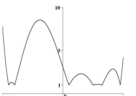
Figure 3 shows a typical Lebesgue function for Lagrange interpolation based on the Chebyshev nodes

T ={xk,n= cos(2k−1)π/(2n) :k= 1,2, . . . , n; n= 1,2,3, . . .}.

(For eachnthese nodes are the zeros of thenth Chebyshev polynomial of the first kind.) The graph illustrates that the maximum of the Lebesgue function on[−1,1]

0 5 10

–1 1

Figure 2: Lebesgue function for Lagrange interpolation on the equally-spaced nodesxk,n= 1−2(k−1)/(n−1) [withn= 9].

occurs at ±1, a result due to Ehlich and Zeller [5]. From the representation Λn(T) =λn(T,±1) = 1

n Xn

i=1

cot(2i−1)π/(4n),

asymptotic results such as Λn(T) = 2

πlogn+2 π

γ+ log8 π

+O

1 n²

(2.2) can be deduced, whereγdenotes Euler’s constant0.577. . .(see [4] for references and more precise results). On comparing (2.1) and (2.2) it can be seen that the Lebesgue constant for Chebyshev nodes ismuchsmaller than for equally-spaced nodes. This confirms the “bad” status of equally-spaced nodes for Lagrange interpolation, a fact that has become well-known largely because of the example of Runge [15].

Figure 3 also suggests that, as withλn(E, x), the local maxima ofλn(T, x)are strictly decreasing from the outside towards the middle of the interval[−1,1]. This was proved by Brutman [3] (see also Günttner [8]).

2.3. Extended Chebyshev nodes

Theextended Chebyshev nodesTbare defined by

Tb={xk,n= cos[(2k−1)π/(2n)]/cos[π/(2n)] :k= 1,2, . . . , n; n= 2,3,4, . . .}.

That is, they are obtained by rescaling the Chebyshev nodes so that the nodes of

0 1 2.5

–1 1

Figure 3: Lebesgue function for Lagrange interpolation on the Chebyshev nodesxk,n= cos (2k−1)π/(2n)[withn= 9].

greatest magnitude for eachnare at±1. Now, it is readily shown that λn(T , x) =b λn(T, xcos[π/(2n)]).

Thus, by the monotonicity result for the local maxima ofλn(T, x), it follows that Λn(T)b is strictly less thanΛn(T)and is equal to the maximum ofλn(T, x)on the interval (cos 3π/(2n),cosπ/(2n)). This characterisation was used by Günttner [9]

to obtain an asymptotic result forΛn(Tb), a simplified version of which is Λn(T) =b 2

πlogn+ 2 π

γ+ log 8 π−2

3

+O 1

logn

. (2.3)

2.4. Augmented Chebyshev nodes

Another modification of T is to add ±1 to each row of the matrix. These augmented Chebyshev nodes Ta are given by x1,n+2 = 1, xn+2,n+2 = −1 and xk,n+2= cos(2k−3)π/(2n)fork= 2,3, . . . , n+ 1.

Now, interpolation polynomials onT andTa are related by Ln+1(Ta, f)(x) =Ln−1(T, f)(x)+

Tn(x)× {(1 +x)[f(1)−Ln−1(T, f)(1)]

+(−1)ⁿ(1−x)[f(−1)−Ln−1(T, f)(−1)]}/2 (2.4)

where Tn(x) = cos(narccosx),−1 6x6 1, is the nth Chebyshev polynomial of the first kind. (To verify (2.4), it is a simple matter to check that the RHS is a polynomial of degree no more than n+ 1which agrees withf at the nodesxk,n+2

for16k6n+ 2.) Thus ifLn(T, f)→f uniformly on[−1,1], thenLn(Ta, f)→f uniformly on[−1,1].

0 1 5

–1 1

Figure 4: Lebesgue function for Lagrange interpolation on the augmented Chebyshev nodes{cos(2k−3)π/(2n) : 26k6n+ 1} ∪ {±1} [withn= 9].

Figure 4 appears to show that the local maximum values ofλn+2(Ta, x)increase from the outside towards the middle of[−1,1](which is the reverse of the situation for T). This was proved by Smith [17], who used essentially the method that was employed by Brutman in [3] to establish the monotonic behaviour of the local maxima ofλn(T, x). Smith also obtained the asymptotic result

Λn+2(Ta) = 4

πlogn+ 4 π

γ+ log4 π

+ 1 +O 1

n²

(2.5) which, when compared with (2.2), shows thatΛn+2(Ta)is effectively doubleΛn(T).

2.5. Optimal nodes

The topic of theoptimal nodesX^∗ for Lagrange interpolation, defined by Λn(X^∗) = min

X Λn(X), n= 2,3,4, . . . ,

has been the subject of much research. Although no explicit formulation ofX^∗ is known, Vértesi [22] showed thatΛn(X^∗)has the asymptotic expansion

Λn(X^∗) = 2

πlogn+2 π

γ+ log4 π

+O log logn logn

2!

. (2.6)

A comparison of (2.3) and (2.6) suggests thatTbis close to optimal. This point is discussed at some length (and made more precise) in Brutman [4, Section 3].

3. Hermite–Fejér interpolation

Given f ∈ C[−1,1] and X defined by (1.2), the Hermite–Fejér interpolation polynomialH2n−1(X, f)of degree2n−1(or less) forf, based onX, is the unique polynomial of degree no greater than 2n−1 which interpolates f and has zero derivative at the nodesxk,n fork= 1,2, . . . , n. It can be written as

H2n−1(X, f)(x) = Xn

i=1

f(xi,n)Ai,n(X, x), (3.1) where the fundamental polynomial Ai,n(X, x) is the unique polynomial of degree no greater than 2n−1 such that Ai,n(X, xk,n) =δi,k and A^′_i,n(X, xk,n) = 0 for k= 1,2, . . . , n.

The Lebesgue function for Hermite–Fejér interpolation onX is λ1,n(X, x) = max

kfk61|H2n−1(X, f)(x)|= Xn

i=1

|Ai,n(X, x)|

and the Lebesgue constant is Λ1,n(X) = max

kfk61kH2n−1(X, f)k= max

−16x61λ1,n(X, x).

For future reference, note that H2n−1(X,1)(x) = 1 (from uniqueness considera- tions), so by (3.1),

Xn

i=1

Ai,n(X, x) = 1. (3.2)

3.1. Chebyshev nodes

Interest in Hermite–Fejér interpolation was sparked by Fejér’s famous 1916 result (see [7]) that if f ∈ C[−1,1], then H2n−1(T, f) converges uniformly to f. Thus there is a simple node system for which the Hermite–Fejér method succeeds for allf ∈C[−1,1], whereas no such system (simple or otherwise) exists for Lagrange interpolation.

A key point in Fejér’s proof is that Ai,n(T, x) > 0 for −1 6 x 6 1 and i = 1,2, . . . n. Thus, by (3.2),

λ1,n(T, x) = Xn

i=1

|Ai,n(T, x)|= Xn

i=1

Ai,n(T, x) = 1,

and so the Lebesgue constantΛ1,n(T)is simply 1.

3.2. A modified Hermite–Fejér method on the augmented Chebyshev nodes

As a “stepping stone” to the study of Hermite–Fejér interpolation on the aug- mented Chebyshev nodes, consider the following interpolation method.

Forn= 1,2,3, . . ., write the Chebyshev nodes as

tk =tk,n= cos(2k−1)π/(2n), k= 1,2, . . . , n,

and let t0 = 1, tn+1 =−1. Givenf ∈C[−1,1], define a polynomialK2n+1(f)of degree2n+ 1(or less) by

( K2n+1(f)(tk) =f(tk), 06k6n+ 1,

K2n+1(f)^′(tk) = 0, 16k6n. (3.3) ThusK2n+1(f)interpolatesf on the augmented Chebyshev nodes and has vanish- ing derivative at the Chebyshev nodes.

An explicit formula forK2n+1(f)in terms of the the Hermite–Fejér interpolation polynomialH2n−1(T, f)is

K2n+1(f)(x) =H2n−1(T, f)(x)+

T_n²(x)× {(1 +x)[f(1)−H2n−1(T, f)(1)]

+(1−x)[f(−1)−H2n−1(T, f)(−1)]}/2. (3.4) (Again, to verify (3.4), it is a simple matter to check that the RHS is a polynomial of degree no more than 2n+ 1 that satisfies the conditions (3.3).) From (3.4) it follows immediately by Fejér’s result that iff ∈C[−1,1], thenK2n+1(f)converges uniformly to f.

Now,K2n+1(f)can also be written in terms of fundamental polynomials as K2n+1(f)(x) =

n+1X

i=0

f(ti)Bi(x),

where for eachi= 0,1, . . . , n+1,Bi(x) =Bi,n(x)is the unique polynomial of degree no greater than 2n+ 1so thatBi(tk) =δi,k fork= 0,1, . . . , n+ 1 andB_i^′(tk) = 0 fork= 1,2, . . . , n. The Lebesgue function and constant are respectively

λn(x) =

n+1X

i=0

|Bi(x)|, Λn = max

−16x61λn(x).

By using elementary properties of the Chebyshev polynomials Tn(x) (see, for example, Rivlin [14, Chapter 1]), it is easy to verify that

B0(x) = 1 +x

2 T_n²(x), Bn+1(x) =1−x

2 T_n²(x) (3.5) and

Bk(x) =(1−x²)(1 +xtk−2t²_k)

n²(x−tk)²(1−t²_k) T_n²(x), 16k6n. (3.6) Observe that for16k6n, the sign ofBk(x)is that of1+xtk−2t²_k. Thus ifn>2, thenB1(x)(for example) is negative for all values ofxin some interval in[−1,1], and so, unlike the Hermite–Fejér method on T, the fundamental polynomials for the modified method are not all non-negative in[−1,1]. In terms of the Lebesgue constant, this means thatΛn>1for alln>2. On the other hand, sinceK2n+1(f) converges uniformly to f for allf ∈C[−1,1], it follows from the uniform bound- edness theorem that theΛn are uniformly bounded. In the following theorem, the best possible bound for theΛn is derived.

Theorem 3.1. The Lebesgue constant Λn satisfies

Λn<3, n= 1,2, . . . (3.7) and

n→∞lim Λn = 3. (3.8)

Proof. By (3.5) and (3.6), λn(x) =T_n²(x)

"

1 + (1−x²) n²

Xn

k=1

|1 +xtk−2t²_k| (x−tk)²(1−t²_k)

# .

Observe that1 +xtk−2t²_k >0if and only ifp(x)< tk < q(x), where p(x) =x−√

x²+ 8

4 , q(x) =x+√ x²+ 8

4 .

LetJn ={1,2, . . . , n}and to givenx∈[−1,1]define

R(x) ={k∈Jn:p(x)< tk < q(x)}, S(x) ={k∈Jn:tk6p(x)ortk >q(x)}. Therefore

λn(x) =T_n²(x)

1 + (1−x²) n² F(x)

, (3.9)

where

F(x) = X

k∈R(x)

1 +xtk−2t²_k

(x−tk)²(1−t²_k)− X

k∈S(x)

1 +xtk−2t²_k (x−tk)²(1−t²_k).

Next employ the partial fraction expansion 1 +xtk−2t²_k

(x−tk)²(1−t²_k)= x

(1−x²)(x−tk)+ 1

(x−tk)² − 1/2

(1−x)(1−tk)− 1/2 (1 +x)(1 +tk).

This leads to F(x) =

Xn

k=1

x

(1−x²)(x−tk)+ 1

(x−tk)² + 1/2

(1−x)(1−tk)+ 1/2 (1 +x)(1 +tk)

− X

k∈R(x)

1

(1−x)(1−tk)+ 1 (1 +x)(1 +tk)

−2 X

k∈S(x)

x

(1−x²)(x−tk)+ 1 (x−tk)²

.

Now, from the identity

T_n^′(x) Tn(x) =

Xn

k=1

1 x−tk

and elementary properties of the Chebyshev polynomials (see, for example, Rivlin [14, Chapter 1]), it follows that

Xn

k=1

1 1−tk

= Xn

k=1

1 1 +tk

=n²

and Xn

k=1

1

(x−tk)² = n²−xTn(x)T_n^′(x) (1−x²)T_n²(x) . Therefore (3.9) becomes

λn(x) = 1 + 2T_n²(x)−2T_n²(x) n²



 X

k∈R(x)

1 +xtk

1−t²_k + X

k∈S(x)

1−xtk

(x−tk)²



. (3.10)

Ifx∈[−1,1]the expression in square brackets is positive, so λn(x)61 + 2T_n²(x), with equality if and only ifTn(x) = 0. In particular,λn(x)<3, from which (3.7) follows.

To establish (3.8), note that it follows from (3.10) that

λ2n(0) = 3− 1 2n²



 X

k∈R(0)

1

1−t²_k + X

k∈S(0)

1 t²_k



, (3.11)

where R(0) = {k ∈ J2n : −1/√

2 < tk < 1/√

2} and S(0) = {k ∈ J2n : tk 6

−1/√

2 ortk >1/√

2}. The sums within the square brackets of (3.11) contain a total of2nterms, each of which is no greater than 2, so

Λ2n>λ2n(0)>3−2 n.

By similar means it can be shown that there exists an absolute constantc so that Λ2n+1>λ2n+1(cos [nπ/(2n+ 1)])>3− c

2n+ 1,

and hence (3.8) is proved.

3.3. Hermite–Fejér interpolation on the augmented Cheby- shev nodes

If f ∈ C[−1,1], then by Fejér’s result, the Hermite–Fejér interpolation poly- nomialsH2n−1(T, f)converge uniformly tof. In Section 3.2 it was shown that if interpolation conditions at ±1 are added to the Hermite–Fejér interpolation con- ditions at the Chebyshev nodes, the resulting interpolation polynomials will still converge uniformly to f. Thus it might be expected that if the full Hermite–Fejér interpolation conditions are applied at±1as well as at the Chebyshev nodes, the resulting polynomialsH2n+3(Ta, f)will converge uniformly tof. Perhaps surpris- ingly, this does not occur.

In fact, Hermite–Fejér interpolation on the augmented Chebyshev nodes ex- hibits some very bad properties! For example, Berman [1] showed that even for f(x) = x², H2n+3(Ta, f)(x) diverges as n → ∞ for all x ∈ (−1,1). (Note that this result doesn’t extend to [−1,1] because ±1 are nodes for all n.) An expla- nation for “Berman’s phenomenon” was provided by R. Bojanić [2], who showed that iff ∈C[−1,1]and the left and right derivativesf_L^′(1)andf_R^′(−1)exist, then H2n−1(Ta, f)→f uniformly if and only if f_L^′(1) =f_R^′(−1) = 0.

Figure 5 shows a typical Lebesgue function λ1,n+2(Ta, x) for Hermite–Fejér interpolation on the augmented Chebyshev nodesTa. On comparing Figures 4 and 5, it appears that the Lebesgue constantΛ1,n+2(Ta)for Hermite–Fejér interpolation is much larger than the Lebesgue constant Λn+2(Ta) for Lagrange interpolation.

This was confirmed by Smith [16], who used methods similar to those employed in the proof of Theorem 3.1 of this paper to show

Λ1,n+2(Ta) =

( 2n²+ 3 +O(1/n), ifnis even, 2n²+ 3−π²/2 +O(1/n), ifnis odd.

4. A weighted interpolation method

In a paper in 1995, Mason and Elliott [12] studied certain weighted interpolation methods based on the zeros of the Chebyshev polynomials of the second, third and

0 170

–1 1

Figure 5: Lebesgue function for Hermite–Fejér interpolation on the augmented Chebyshev nodes{cos(2k−3)π/(2n) : 26k6n+ 1} ∪ {±1} [withn= 9].

fourth kinds. Although the resulting interpolating functions are not polynomials, there are many similarities between the study of these functions and the study of Lagrange interpolation polynomials. We illustrate Mason and Elliott’s ideas by discussing their weighted interpolation method based on the zeros of Chebyshev polynomials of the second kind.

Denote the set of algebraic polynomials of degree at mostn by Πn, let w(x) denote the weight function w(x) =√

1−x², and let X and xi,n be given by (1.1) and (1.2) with xi,n 6= ±1. We consider the interpolating projection Pn−1(X) of C[−1,1]onwΠn−1 that is defined by

Pn−1(X)(f)(x) =w(x) Xn

i=1

f(xi,n)ℓi,n(X, x)/w(xi,n). (4.1)

Also defineθk =θk,n=kπ/(n+ 1)and put

U ={xk,n= cosθk,n:k= 1,2, . . . , n; n= 1,2,3, . . .}.

(Thus for fixed n, thexk,n are the zeros of the nth Chebyshev polynomial of the second kind.)

Mason and Elliott showed that the projection norm (or Lebesgue constant) kPn−1(U)k= max

kfk61kPn−1(U)(f)k

has the representation

kPn−1(U)k= max

06θ6πFn(θ), where

Fn(θ) =|sin(n+ 1)θ| n+ 1

Xn

i=1

sinθi

cosθ−cosθi

.

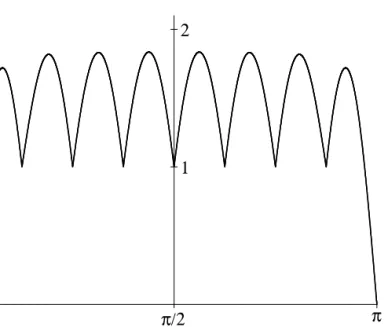
Based on numerical computations, Mason and Elliott conjectured that the maxi- mum ofFn(θ)occurs atπ/2for evennand asymptotically atnπ/(2n+ 2)(which is midway between the θ-nodes of θ(n−1)/2 and θ(n+1)/2 =π/2) for odd n. This conjecture is supported by the graph ofF7(θ)in Figure 6.

1

π/2 π 0

2

Figure 6: Plot ofF7(θ)

Now, assuming that their conjecture about the maximum of Fn(θ) is true, Mason and Elliott showed that

kPn−1(U)k= 2

πlogn+ 2 π

γ+ log 4 π

+o(1). (4.2)

Smith [18] later established the validity of (4.2), although the proof did not depend on Mason and Elliott’s conjecture (which remains unresolved). The result (4.2) means that, to within o(1) terms, kPn−1(U)k is equal to Λn(X^∗), the smallest possible Lebesgue constant forunweightedLagrange interpolation (see Section 2.5).

Furthermore, by a result of Kilgore [10], the minimum ofkPn−1(X)k over allX is no smaller thanΛn(X^∗). Thus

minX kPn−1(X)k=kPn−1(U)k+o(1),

which means that for the weighted interpolation method defined by (4.1), there is a simple description of nodes that are essentially optimal.

Acknowledgements. The author thanks the Department of Mathematics and Statistics of La Trobe University and the Analysis Department of the Rényi Math- ematical Institute, Budapest (OTKA T037299) for financial support to attend the Fejér–Riesz conference in Eger in June 2005, where a talk based on a draft version of this paper was presented.

References

[1] Berman, D. L.,A study of the Hermite–Fejér interpolation process,Doklady Akad.

Nauk USSRVol. 187 (1969), 241–244 (in Russian) [Soviet Math. Dokl.Vol. 10 (1969), 813–816].

[2] Bojanić, R.,Necessary and sufficient conditions for the convergence of the extended Hermite–Fejér interpolation process,Acta Math. Acad. Sci. Hungar.Vol. 36 (1980), 271–279.

[3] Brutman, L., On the Lebesgue function for polynomial interpolation, SIAM J.

Numer. Anal.Vol. 15 (1978), 694–704.

[4] Brutman, L., Lebesgue functions for polynomial interpolation — a survey,Ann.

Numer. Math.Vol. 4 (1997), 111–127.

[5] Ehlich, H., Zeller, K., Auswertung der Normen von Interpolationsoperatoren, Math. Ann.Vol. 164 (1966), 105–112.

[6] Faber, G.,Über die interpolatorische Darstellung stetiger Funktionen, Jahresber.

der Deutschen Math. Verein.Vol. 23 (1914), 192–210.

[7] Fejér, L.,Ueber Interpolation,Göttinger Nachrichten(1916), 66–91.

[8] Günttner, R.,Evaluation of Lebesgue constants,SIAM J. Numer. Anal.Vol. 17 (1980), 512–520.

[9] Günttner, R.,On asymptotics for the uniform norms of the Lagrange interpolation polynomials corresponding to extended Chebyshev nodes, SIAM J. Numer. Anal.

Vol. 25 (1988), 461–469.

[10] Kilgore, T.,Some remarks on weighted interpolation, in N. K. Govilet al., eds, Approximation Theory(Marcel Dekker, New York, 1998) pp. 343–351.

[11] Luttmann, F. W., Rivlin, T. J., Some numerical experiments in the theory of polynomial interpolation,IBM J. Res. Develop.Vol. 9 (1965), 187–191.

[12] Mason, J. C., Elliott, G. H., Constrained near-minimax approximation by weighted expansion and interpolation using Chebyshev polynomials of the second, third, and fourth kinds,Numer. AlgorithmsVol. 9 (1995), 39–54.

[13] Rivlin, T. J., An Introduction to the Approximation of Functions, Dover, New York, 1981.

[14] Rivlin, T. J.,Chebyshev Polynomials: From Approximation Theory to Algebra and Number Theory, 2nd ed. Wiley, New York, 1990.

[15] Runge, C.,Über empirische Funktionen und die Interpolation zwischen äquidistan- ten Ordinaten,Z. für Math. und Phys.Vol. 46 (1901), 224–243.

[16] Smith, S. J., The Lebesgue function for Hermite–Fejér interpolation on the ex- tended Chebyshev nodes,Bull. Austral. Math. Soc.Vol. 66 (2002), 151–162.

[17] Smith, S. J.,The Lebesgue function for Lagrange interpolation on the augmented Chebyshev nodes,Publ. Math. DebrecenVol. 66 (2005), 25–39.

[18] Smith, S. J.,On the projection norm for a weighted interpolation using Chebyshev polynomials of the second kind,Math. Pannon.Vol. 16 (2005), 95–103.

[19] Szabados, J., Vértesi, P.,Interpolation of Functions, World Scientific, Singapore, 1990.

[20] Tietze, H.,Eine Bemerkung zur Interpolation,Z. Angew. Math. and Phys.Vol. 64 (1917), 74–90.

[21] Turetskii, A. H.,The bounding of polynomials prescribed at equally distributed points,Proc. Pedag. Inst. VitebskVol. 3 (1940), 117–127 (in Russian).

[22] Vértesi, P.,Optimal Lebesgue constant for Lagrange interpolation,SIAM J. Nu- mer. Anal.Vol. 27 (1990), 1322–1331.

Simon J. Smith

Department of Mathematics and Statistics La Trobe University

P.O. Box 199, Bendigo, Victoria 3552 Australia