Fuzzy Interpolation According to Fuzzy and Classical Conditions

Fuzzy Interpolation According to Fuzzy and Classical Con- ditions

I. Perfilieva, M. Wrublov´a, P. Ho ˇd´akov´a

University of Ostrava, Inst. for Research and Applications of Fuzzy Modeling 30. dubna 22, 701 03 Ostrava 1, Czech Republic

e-mail:{Irina.Perfilieva,Michaela.Wrublova,Petra.Hodakova}@osu.cz

We will be focused on the interpolation approach to a computation with fuzzy data. A definition of interpolation of fuzzy data, which stems from the classical approach, is proposed. We investigate another approach to fuzzy interpolation (published in [5]) with relaxed interpolation condition. We prove that even if the interpolation condition is relaxed the related algorithm gives an interpolating fuzzy function which fulfils the interpolation condition in the classical sense.

Keywords: Fuzzy function; fuzzy equivalence, fuzzy space, fuzzy interpolation, fuzzy rule base interpolation

1 Introduction

In the following, we will deal with a problem of a fuzzy interpolation. We will first recall a classical approach to interpolation, because the problem of fuzzy interpolation closely relates to it.

Letf be a real function of a real argument with a domain M = {x_i, i = 1, . . . , n} ⊂ R, and {(xi, f(xi)), i= 1, . . . , n} ⊆Rbe the interpolation data. LetM ⊂P ⊆R. An interpolation function g:P −→Ris a function that fulfils the interpolation condition:

f(xi) =g(xi), i= 1, . . . , n.

In this paper, we will be focused on the interpolation approach to a computation with fuzzy data. A precise definition ofinterpolation of fuzzy datawill be given below in the subsection 2.4. Freely speaking, this is a problem of extension of a fuzzy function given on a restricted domain to a fuzzy function given on a wider domain (similar to the case considered above).

There are other approaches to the problem of fuzzy interpolation. They differ one from the other one by restrictions on interpolation functions. The following list remembers the most popular approaches : level cuts interpolation [17, 18], analogy-based interpolation [3, 4, 6], interpolation by convex completion [8, 23], interpolation by geometric transformations [1], interpolation in a family of interpolating relations [2], polar cut interpolation [15], interpolation based on closeness relations [5], flank functions interpolation [13, 14], analytic fuzzy relation-based interpolation [20], and fuzzy interpolation based on fuzzy functions [11].

The sections below are arranged as follows : basic concepts as well as definition of fuzzy interpolation will be given in Section 2. In Section 3, we will recall the approach to fuzzy interpolation introduced by Godo, Esteva, ets. in [5]. The last Section 4 is devoted to a new approach.

2 Fuzzy Interpolation and Its Analytic Representation

In this section, we will introduce the problem of fuzzy interpolation as a problem of extension of a partially given fuzzy function. Moreover, we expect that a solution will be represented analytically with the help of a structure known as residuated lattice.

First of all, we will recall the notion of residuated lattice, then we will introduce the notion of fuzzy space and fuzzy function. Finally, we will discuss a certain class of interpolating fuzzy functions and their analytical representation.

2.1 Residuated Lattice

A residuated lattice is an ordered algebraic structure with two residuated binary operation. We will recall its definition from [19].

Definition 1

A residuated lattice^∗)is an algebra

L=hL,∨,∧,∗,→,0,1i.

with a supportLand four binary operations and two constants such that

• hL,∨,∧,0,1iis a lattice where the ordering≤defined using operations∨,∧as usual, and0,1are the least and the greatest elements, respectively;

• hL,∗,1iis a commutative monoid, that is,∗ is a commutative and associative operation with the identitya∗1=a;

• the operation→is a residuation operation with respect to∗, i.e., a∗b≤c iff a≤b→c.

A residuated lattice is complete if its underlying lattice is complete.

The derived operation is biresiduum:

a↔b= (a→b)∧(b→a).

Our investigation will be based on Łukasiewicz algebraLŁ. It is a residuated lattice with the support L= [0,1]where

a∗b= 0∨(a+b−1), a→b= 1∧(1−a+b), a↔b= 1− |a−b|.

The other well known examples of residuated lattice are Boolean algebra, G¨odel algebra and product algebra.

2.2 L-fuzzy Space

Assume that we are given a complete residuated latticeLand a non-empty universal setX ⊆RwhereRis the set of real numbers. AnL-valued fuzzy setis a mappingA:X →L. Acoreof a fuzzy setAis the set Core(A) ={x∈X|A(x) = 1}. We say that a fuzzy set isnormalif there existsxA ∈X : A(xA) = 1.

The class ofL-valued fuzzy sets ofXwill be denoted byL^X.

LetA, B∈L^Xbe fuzzy sets. Afuzzy equality(A≡B)is given by the following formula (A≡B) = ^

x∈X

(A(x)↔B(x))^†). (1)

∗)In this paper we assume a residuated lattice to be bounded, commutative and integral.

†)for a general definition of fuzzy equality, e.g., [7, 12, 16]

The fuzzy equality determines a degree of coincidence of two fuzzy sets expressed by an element of the residuated lattice.

It is known that

(A≡B) = 1 iff ∀x∈X, A(x) =B(x), In this case we will writeA=Binstead ofA≡B.

Definition 2

The pair(L^X,≡)is a fuzzy space onX.

The definition of fuzzy space introduces a basic set of objects together with the basic relation of equal- ity.

Example 1

LetX = [a, b], L = LŁ. Let us show how the fuzzy equality≡is expressed. Assume that A, B ∈ [0,1]^[a,b].

A≡B= ^

x∈[a,b]

(A(x)↔B(x)) = ^

x∈[a,b]

(1− |A(x)−B(x)|) =

1− _

x∈[a,b]

|A(x)−B(x)|. Thus the pair([0,1]^[a,b], 1−W

x∈[a,b]|A(x)−B(x)|)is a fuzzy space on[a, b]determined by Łukasiewicz algebra.

In the special case where fuzzy sets on[a, b]are continuous mappings, the fuzzy equality≡between them can be simplified to

1− _

x∈[a,b]

|A(x)−B(x)|= 1− max

x∈[a,b]|A(x)−B(x)|= 1−d(A, B), whered(A, B)is the distance in the metric space of continuous functions.

2.3 Fuzzy Function

We will use the notion of fuzzy function introduced in [20]. According to [20], a fuzzy function is an ordinary mapping between two fuzzy spaces. In more details,

Definition 3

LetLbe a complete residuated lattice and(L^X,≡),(L^Y,≡)fuzzy spaces onX andY, respectively. A mappingf :L^X−→L^Y is a fuzzy function if for everyA, B∈L^X,

A=Bimpliesf(A) =f(B). (2)

Let us remark that there are other definitions of fuzzy function in [7, 9, 10, 16] where fuzzy function is defined as a fuzzy set of function or as a special fuzzy relation.

Below, we give an example of a fuzzy function which is reproduced from [21].

Example 2 (Fuzzy functions determined by a fuzzy relation)

Let(L^X,≡),(L^Y,≡)be fuzzy spaces onX andY respectively,R∈L^X×Y a fuzzy relation. For every A∈L^X, we define the◦-compositionofAandRby

(A◦R)(y) = _

x∈X

(A(x)∗R(x, y)). (3)

Composition (3) determines the fuzzy setA◦RonY. The corresponding mappingf_◦R:A7→A◦Ris a fuzzy function defined on the whole fuzzy spaceL^X.

2.4 Fuzzy Interpolation

The problem of fuzzy interpolation includes two subproblems: a choice of a set of interpolation functions and an extension of an original fuzzy function.

In other words, let{(Ai, Bi), i = 1, . . . , n} be a set of fuzzy data andAi ∈ L^X, i = 1, . . . , nare pairwise different fuzzy sets with respect to=,Bi ∈L^Y, i= 1, . . . , n. Let a fuzzy functionf : Ai → Bi, i = 1, . . . , nhave the domain M = {A1, . . . , An}, andP be a domain of an interpolation fuzzy functiongwhereM ⊂P ⊆L^X. LetN ⊆ {g|g: P −→L^Y}be a chosen subset of a fuzzy function for the fuzzy interpolation. Our goal is to find an fuzzy functiong∈ N satisfying the interpolation condition

g(A_i) =B_i, i= 1, . . . , n. (4) The fuzzy functiongis calledan interpolation fuzzy functionfor fuzzy data. Also we call the interpolation fuzzy functiongan extension offon the domainP.

We can also rewrite the interpolation condition (4) as follows:

A=Aiimpliesg(A) =Bi, i= 1, . . . , n. (5)

2.5 Similarity and Fuzzy Point

A binary fuzzy relationE onXis called a similarity onX if for allx, y, z∈X, the following properties hold:

1. E(x, x) = 1, 2. E(x, y) =E(y, x),

3. E(x, y)∗E(y, z)≤E(x, z).

LetEbe a similarity onX. A fuzzy setE_t, t∈X, whereE_t(x) =E(t, x)for allx∈Xis called an E-fuzzy pointofX.

3 Fuzzy Rule Base Interpolation

In this contribution, we will investigate another approach to fuzzy interpolation, proposed in [5]. It assumes that an original function is expressed by a set of fuzzy IF-THEN rules

RB={“IfxisAithenyisBi”}i=1,...,n (6) (AiandBiare respective fuzzy sets onX andY), and the rules are sparse in the sense thatAi∩Aj=∅, i 6= j. The fuzzy interpolation is proposed to be realized in a form of an algorithm which produces a consequence B to an antecedenceA (A andB are fuzzy sets too). An interpolating algorithm should respect the following requirement:

“The more the inputAisclose toAi

the more the outputBmust beclose toBi.” (7) In [5], a general interpolating algorithm is proposed. Below, we give its essential details that char- acterize relations of closeness on both universes and describe the way of computingB according to the requirement (7).

The closeness relations between two fuzzy sets show how much one is similar or is included into the other one. LetS={Sλ; 0≤λ≤ +∞}, be any nested family of fuzzy similarity relations onRsuch that S0is the crisp equality andS_+∞=1. Then

closeλ(E, D) =min(IS_λ(D|E), IS_λ(E|D)), (8) where

IS_λ(D|E) =inf_u∈R{E(u)→(Sλ◦D)(u)}. (9) According to [5], the value of (algorithmically defined) interpolating function at pointAis fuzzy setB such that

B=Interpol_RB(A) =∩R_i∈K(A)∩λ≥0closeλ(A, A_i)→(S_f(λ)◦B_i), (10) whereK(A)is a subset of fuzzy rules related toA,→is the residuum of a left-continuous t-norm∗, and◦ is the max-* composition. Moreover, for each0< λ≤+∞,

f(λ) =inf{µ|closeλ(A1, A2)≤closeµ(B1, B2)}, (11) whereµis any parameter which satisfies the inequality closeλ(A1, A2)≤closeµ(B1, B2). It is proved in [5] that thus proposed algorithm fulfils the requested requirement (7).

It is seen from the description above, that a specification of the algorithm requires a choice of a para- metric family of fuzzy similarity relationsSand operations from a certain residuated lattice. One partial specification was proposed in [5] as well. It is based on an arbitrary left-continuous t-norm∗ and the parametric family of fuzzy similarity relations onR²:

Sλ(x, y) =max(1−|x−y|

λ ,0). (12)

4 Main Result

Our purpose it to show that the interpolation algorithm presented in [5] and based on the fuzzy prescrip- tion (7) satisfies the interpolation condition in the sense (4). It means that the interpolation function Interpol_RB(A)(cf. (10)) fulfils the interpolation condition in the form

(∀Ai) Interpol_RB(Ai) = Bi, i= 1, . . . , n.

4.1 Assumptions and Preliminaries

The Łukasiewicz algebra is chosen as an underlying residuated lattice. Without lost of generality, we assume that only two IF-THEN fuzzy rules specify an original function so that the subset of IF-THEN fuzzy rules connected withAis

K(A) ={A1→B1, A2→B2}.

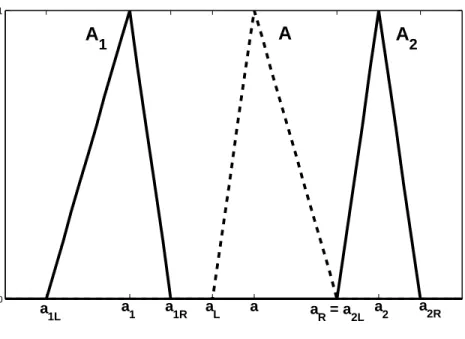
LetA1, A2be normal and triangular shaped fuzzy sets (inputs) defined onX ⊂RandB1, B2be normal and triangular shaped fuzzy sets (outputs) defined onY ⊂R. Obviously, the core of a triangular shaped fuzzy set consists of one element – thecore point. Denote core points ofA1, A2byxA₁ andxA₂, and similarly, core points ofB1, B2 byyB₁ andyB₂, respectively. Denote (arbitrary) normal and triangular shaped fuzzy set onX ⊂RbyA, and its core point byxA. Our aim is to prove that the fuzzy setBgiven by (10) fulfils (4).

LetSλ be a similarity onX andλ ≥ 0a fixed real number. The composition betweenSλandAis given by

(Sλ◦A)(x) =_

u

(Sλ(x, u)∗A(u)).

In the following proposition we will show how the similarity relationSλaffects a fuzzy set.

0 1

A

A A

1

a1L a

1 a

1R a

L a a_R = a_2L a

2 a

2R

Figure 1: Fuzzy sets onX Proposition 1

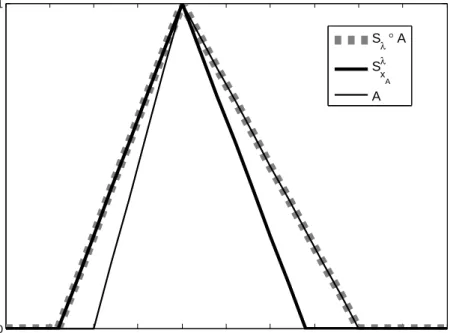
LetAbe a normal fuzzy set and xA ∈ X be its core point. Let moreover, S_x^λ_A be the Sλ-fuzzy point determined byx_A, i.e.S^λ_x

A =S_λ(x_A, x). Then for allx∈X: 1. (S_λ◦A)(x)≥A(x),

2. (Sλ◦A)(x)≥S_x^λ_A(x),

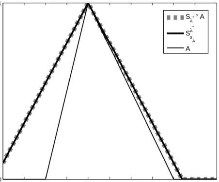
3. there existsλ^∗≥0such thatA(x)≤S_x^λ∗

A(x)and then(S_λ^∗◦A)(x) =S_x^λ∗

A(x).

PROOF

:

1. (Sλ◦A)(x) =W

u(Sλ(x, u)∗A(u))≥(Sλ(x, x)∗A(x)) =A(x).

2. (Sλ◦A)(x) =W

u(Sλ(x, u)∗A(u))≥(Sλ(x, xA)∗A(xA)) =Sλ(x, xA) =Sλ(x, xA) =S_x^λ_A(x).

3. Assume thatA(u)≤S_x^λ_A^∗(u)so that the following holds:(Sλ^∗◦A)(x) =W

u(Sλ^∗(x, u)∗A(u))≤ W

u(Sλ^∗(x, u)∗Sλ^∗(xA, u)) =W

u(Sλ^∗(x, u)∗Sλ^∗(u, xA)) =Sλ^∗(x, xA) =Sλ^∗(xA, x). On the other side,(S_λ∗◦A)(x)≥S_x^λ∗

A(x)forλ^∗≥0. Therefore,(S_λ∗◦A)(x) =S_x^λ∗

A(x).

2

By the proposition above, we can rewrite (8) as follows:

closeλ(A₁, A₂) =min(I_Sλ∗(A₂|A1), I_Sλ∗(A₁|A2)) =

=^

x

(S_λ^∗◦A₁↔S_λ^∗◦A₂) where

IS_λ(A2|A1) =infx∈R{A1(u)→(Sλ^∗◦A2)(u)}=

=inf_x∈R{Sλ^∗(xA₁, x)→Sλ^∗(xA₂, x)},

0 1

S_λ ° A S^λ

x A

A

Figure 2: Properties(Sλ◦A)(x)≥A(x)and(Sλ◦A)(x)≥S_x^λ_A(x)

and similarlyIS_λ(A1|A2).

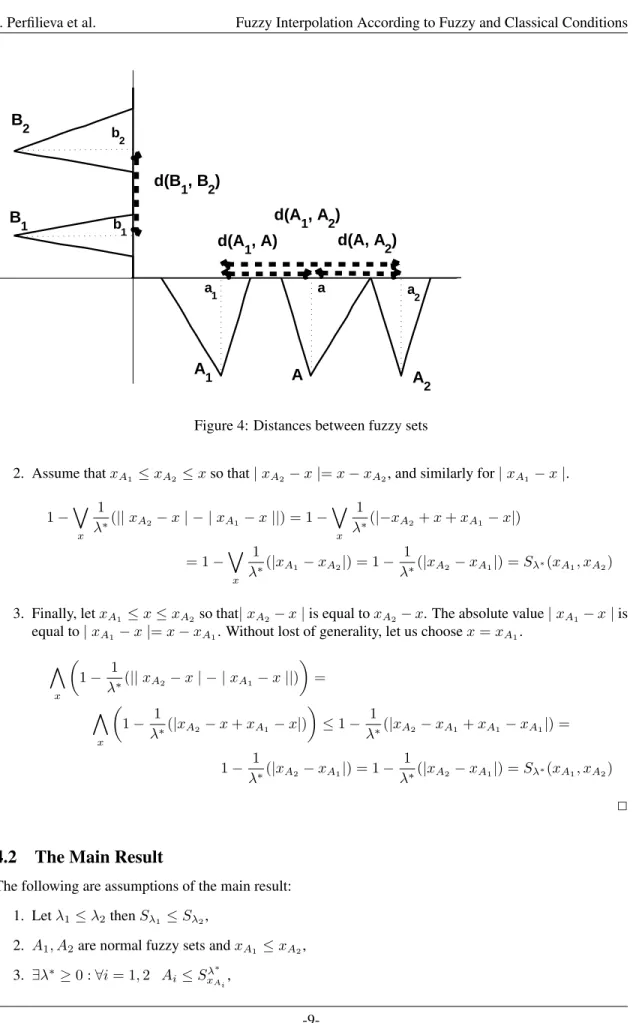
Let us simplify the expression (10) by applying assumptions that are accepted at the beginning of this subsection. Moreover, we replace similarities by distances (similar approach has been used in [22]). The distance between two triangular shaped fuzzy sets is considered as a distance between their core points^‡):

d(A, A₁) =|x_A−x_A1|, d(A, A2) =|x_A−x_A2 |, d(A1, A2) =|xA₁−xA₂ |

and

d(B1, B2) =|yB₁−yB₂ |. Proposition 2

LetA1, A2be normal and triangular shaped fuzzy sets withxA₁, xA₂ ∈Xas respective cores. LetSλ^∗

be given by (12), andλ^∗≥0. Then

^

x

(S_λ^∗◦A₁↔S_λ^∗◦A₂) =S_λ^∗(x_A1, x_A2).

PROOF

:

−(||a| − |b||)≥ −(|a| − |b|).

‡)Recall that each triangular shaped fuzzy set has exactly one core point so that our definition of a distance is correct.

0 1

Sλ^* ° A S^λ

* xA

A

Figure 3: PropertyA(x)≤S^λ_xA^∗(x),(Sλ^∗◦A)(x) =S_x^λ_A^∗(x)

^

x

(S_λ∗◦A₁↔S_λ∗◦A₂) =^

x

(S_x^λ∗

A1(x)↔S^λ_x^∗

A2(x)) =^

x

(1− |S_λ∗(x_A1, x)−

Sλ^∗(xA₂, x)|) =^

x

1−

1−|xA₁−x|

λ^∗ −1 +|xA₂−x| λ^∗

=

^

x

1−

|xA₂−x|

λ^∗ −|xA₁−x| λ^∗

=^

x

1− 1

λ^∗||xA₂−x| − |xA₁−x||

= 1−_

x

1

λ^∗(||xA2−x| − |xA1−x||)≥1−_

x

1

λ^∗(|xA2−x−xA1+x|) = 1−_

x

1

λ^∗(|xA₂−xA₁|) = 1− 1

λ^∗(|xA₂−xA₁|) =Sλ^∗(xA₁, xA₂) Assume thatx≤x_A1≤x_A2. Three cases are possible.

1. x≤xA₁ ≤xA₂. In this case,|xA₂−x|=xA₂−x. Similarly for|xA₁−x|.

1−_

x

1

λ^∗(||xA2−x| − |xA1−x||) = 1−_

x

1

λ^∗(|xA2−x−xA1+x|)

= 1−_

x

1

λ^∗(|xA₂−xA₁|) = 1− 1

λ^∗(|xA₂−xA₁|) =Sλ^∗(xA₁, xA₂)

a1 a a 2

d(A1, A

2)

A A

1 A

2

B1

B2

b1

b2

d(B1, B

2)

d(A, A

2) d(A1, A)

Figure 4: Distances between fuzzy sets

2. Assume thatxA₁ ≤xA₂ ≤xso that|xA₂−x|=x−xA₂, and similarly for|xA₁−x|.

1−_

x

1

λ^∗(||xA₂−x| − |xA₁−x||) = 1−_

x

1

λ^∗(|−xA₂+x+xA₁−x|)

= 1−_

x

1

λ^∗(|xA1−x_A2|) = 1− 1

λ^∗(|xA2−x_A1|) =S_λ^∗(x_A1, x_A2) 3. Finally, letx_A1 ≤x≤x_A2so that|x_A2−x|is equal tox_A2−x. The absolute value|x_A1−x|is

equal to|xA₁−x|=x−xA₁. Without lost of generality, let us choosex=xA₁.

^

x

1− 1

λ^∗(||xA₂−x| − |xA₁−x||)

=

^

x

1− 1

λ^∗(|xA2−x+x_A1−x|)

≤1− 1

λ^∗(|xA2−x_A1+x_A1−x_A1|) = 1− 1

λ^∗(|xA₂−xA₁|) = 1− 1

λ^∗(|xA₂−xA₁|) =Sλ^∗(xA₁, xA₂) 2

4.2 The Main Result

The following are assumptions of the main result:

1. Letλ₁≤λ₂thenS_λ1 ≤S_λ2,

2. A1, A2are normal fuzzy sets andxA₁≤xA₂, 3. ∃λ^∗≥0 :∀i= 1,2 Ai≤S_x^λ∗

Ai,

4. S_x^λ_A^∗

1 ∧S_x^λ_A^∗

2 = 0.

We will describe and concretize the other parts of the expression (10) by means of distances.

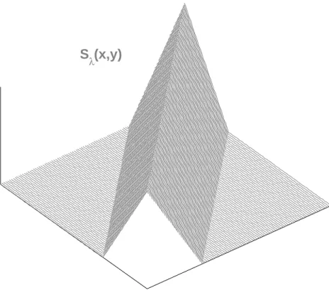
Letλ^∗≤λ≤+∞. Let us remind that the same parametric family of fuzzy similarity relations onR² is given by (12).

S

(x,y)

Figure 5: Similarity relation

The idea is that we extend the fuzzy setA1by applying to itSλwhereλ^∗≤λ≤+∞.

Now we rewrite the expression (8) (degree of closeness) using distances. For each0< λ≤+∞, closeλ(A1, A2) =min(IS_λ(A2|A1), IS_λ(A1|A2)) = λ− |xA1−xA2 |

λ , (13)

and respectively,

closeλ(A, Ai) =λ− |x_A−x_Ai |

λ , i= 1,2. (14)

The respective valuef(λ)can now be expressed as

f(λ) = λ|yB₁−yB₂ |

|x_A1−x_A2 | . (15)

The expression (15) is equivalent to (11). However, (15) is represented with the help of distances and by this, its meaning is clearer.

−3 −2 −1 0 1 2 3 4 5 6 7 0

0.1 0.2 0.3 0.4 0.5 0.6 0.7 0.8 0.9 1

A₁ A₂ S_λ°A₁

Figure 6: Extension fuzzy setA1

Finally, we will characterize the fuzzy setBgiven by (10) with the help of distances too.

B=

2

^

i=1

^

λ

(closeλ(A, Ai)→(S_f(λ)◦Bi)(y)) =

2

^

i=1

^

λ

1−1 + |x_A−x_Ai |

λ + (S_f(λ)◦B_i)(y)

=

2

^

i=1

^

λ

|xA−xA_i |

λ + (S_f(λ)◦Bi)(y)

Now, we can prove that the interpolation condition (5) is fulfilled.

Theorem 1

IfA=AithenB =Bifori= 1,2.

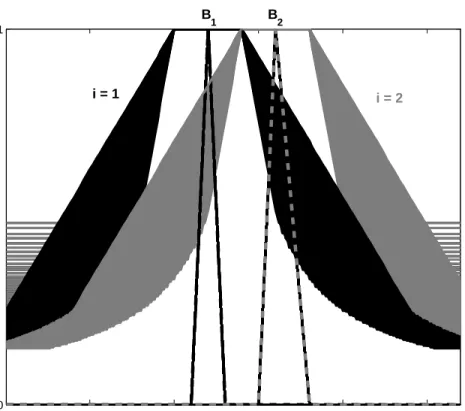
0 1

B₁ B₂

i = 1 i = 2

Figure 7: Construction of output fuzzy setB PROOF

:

B=

2

^

i=1

^

λ

(closeλ(A, Ai)→(S_f(λ)◦Bi)(y)) =

2

^

i=1

^

λ

0∨

1−1 + |x_A−x_Ai |

λ + (S_f(λ)◦B_i)(y)

=

2

^

i=1

^

λ

0∨

|xA−xA_i |

λ + (S_f(λ)◦Bi)(y)

=

"

^

λ

|x_A−x_A1 |

λ + (S_f(λ)◦B₁)(y) #

^

"

^

λ

|xA−xA₂ |

λ + (S_f(λ)◦B2)(y) #

=B⁰∧B⁰⁰ For eachi= 1,2, we will prove thatA=A_i ⇒ B=B_i.

LetA=A1. B⁰ =^

λ

(closeλ(A1, A1)→(S_f(λ)◦B1)(y)) =

^

λ

|xA₁−xA₁ |

λ + (S_f(λ)◦B1)(y)

=

^

0<λ≤λ⁰

|xA₁−xA₁ |

λ + (S_f(λ)◦B1)(y)

∧

^

λ>λ⁰

|xA₁−xA₁|

λ + (S_f(λ)◦B1)(y)

=

^

0<λ≤λ⁰

0 + (S_f(λ)◦B1)(y)

∧ ^

λ>λ⁰

0 + (S_f(λ)◦B1)(y)

=

B1(y)∧

"

^

λ>λ⁰

0 + (Sf(λ)◦B1)(y)

#

=B1(y)∧

"

^

λ>λ⁰

(Sf(λ)(yB₁, y)

#

=B1

The latter equality follows fromV

0<λ≤λ⁰ (S_f(λ)◦B1)(y)

=B1which can be justified by the fol- lowing chain of inequalities:

f(λ⁰)≤|y_B1−y|, λ⁰|yB₁−yB₂ |

|xA₁−xA₂ | ≤|yB₁−y|, λ⁰|yB₁−yB₂ |

|x_A1−x_A2 | ≤|yB₁−y|, λ⁰≤|y_B1−y| |x_A1−x_A2|

|yB₁−yB₂|.

B⁰⁰=^

λ

(closeλ(A1, A2)→(S_f(λ)◦B2)(y)) =

^

λ

|xA₁−xA₂ |

λ + (S_f(λ)◦B2)(y)

=

^

λ

|xA₁−xA₂ |

λ + (1−|yB₂−y| f(λ) ∨0)

=

^

λ

1 +|xA₁−xA₂|

λ −|yB₂−y| f(λ)

=

^

λ

1−

|yB₂−y|

f(λ) −|xA₁−xA₂ | λ

=

^

λ



1−





|y_B2−y|

λ|yB1−yB2|

|xA1−xA2|

−|x_A1−x_A2 | λ







=

^

λ

1−

|y_B2−y||x_A1−x_A2|

λ|yB₁−yB₂ | −|x_A1−x_A2| λ

=

^

λ

1−1

λ

|y_B2−y||x_A1−x_A2 |

|yB₂−yB₁ | − |xA1−xA2 |

=

^

λ

1− 1

λ

(yB2−y)(xA1−xA2) (yB₂−yB₁)

− |xA₁−xA₂ |

≥

^

λ

1− 1

λ

(yB₂−y)(xA₁−xA₂)−((xA₁−xA₂)(yB₂−yB₁)) (yB₂−yB₁)

=

^

λ

1− 1

λ

−y(xA₁−xA₂) +xA₁yB₁−xA₂yB₁

(yB₂−yB₁)

=

^

λ

1−1

λ

yB₁(xA₁−xA₂)−y(xA₁−xA₂) (y_B2−y_B1)

=

^

λ

1− 1

λ

(xA₁−xA₂)(yB₁−y) (y_B2−y_B1)

=

^

λ

1−1

λ

(xA₁−xA₂) (y_B2−y_B1)

|y_B1−y|

=

^

λ

1−1

λ

(x_A1−x_A2) (yB₁−yB₂)

(|y_B1−y|)

=

^

λ

1− 1

f(λ)(|(y_B1−y)|)

∨0

=

^

λ

Sf(λ)◦B1

Finally,

A=A1⇒B=B⁰∧B⁰⁰=B1∧B⁰⁰=B1, whereB⁰⁰≥V

λ Sf(λ)◦B1

andV

λ Sf(λ)◦B1

=B1. Similarly forA=A₂.

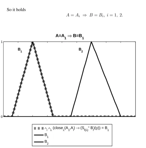
So it holds

A=Ai ⇒ B =Bi, i= 1, 2.

2

0 1

A=A₁ ⇒ B=B₁

∧_i ∧_λ (close_λ(A

1,A

i) → (S_f(λ)° B_i)(y)) = B

1

B1

B₂

B1 B

2

Figure 8: Interpolation condition,A=A1→B=B1

Acknowledgement

The paper has been partially supported by the grant “F-transform in various aspects of image processing”

of the M ˇSMT ˇCR.

Conclusions

We have proposed a definition of interpolation of fuzzy data, which stems from the classical approach based on rigorous interpolation condition. We investigated another approach to fuzzy interpolation (published in [5]) with relaxed interpolation condition. We simplified and illustrated in various pictures the interpolation algorithm that is based on the proposed in [5] approach. We proved that even if the interpolation condition is relaxed the related algorithm gives an interpolating fuzzy function which fulfils the interpolation condition in the classical sense. Thus the interpolation algorithm in [5] is in the agreement with the definition of interpolation of fuzzy data which we proposed.

0 1

A = A

2⇒ B = B

2

∧_i ∧_λ(close_λ(A

2,A

i) → (S_f(λ)° B_i)(y)) = B

2

B1

B2

B1 B

2

Figure 9: Interpolation condition,A=A₂→B=B₂

References

[1] P. Baranyi, T. D. Gedeon, Rule interpolation by spatial geometric representation, in: Proc. of IPMU’96 Conf., Granada, 1996.

[2] P. Baranyi, L. T. K´oczy, T. D. Gedeon, A generalized concept for fuzzy rule interpolation, IEEE Transactions on Fuzzy Systems 12 (2004) 820–837.

[3] B. Bouchon-Meunier, J. Delechamp, C. Marsala, N. Mellouli, M. Rifqi, L. Zerrouki, Analogy and fuzzy interpolation in case of sparse rules, in: Proc. of the EUROFUSE-SIC Joint Conf., 1999.

[4] B. Bouchon-Meunier, D. Dubois, C. Marsala, H. Prade, L. Ughetto, A comparative view of interpo- lation methods between sparse fuzzy rule, in: Proc. of the Joint 9th IFSA World Congress and 20th NAFIPS International Conference, 2001.

[5] B. Bouchon-Meunier, F. Esteva, L. Godo, M. Rifqi, S. Sandri, A principled approach to fuzzy rule base interpolation using similarity relations, in: Proc. of the EUSFLAT-LFA Joint Conf., 2005.

[6] B. Bouchon-Meunier, C. Marsala, M. Rifqi, Interpolative reasoning based on graduality, in: Proc. of FUZZ-IEEE’2000 Int. Conf., San Antonio, 2000.

[7] M. Demirci, Fundamentals of m-vague algebra and m-vague arithmetic operations, Int. Journ. Uncer- tainty, Fuzziness and Knowledge-Based Systems 10 (2002) 25–75.

[8] D. Dubois, R. Martin-Clouaire, H. Prade, Practical computing in fuzzy logic, in: M. M. Gupta, T. Yamakawa (eds.), Fuzzy Computing, North-Holland, 1988.

[9] D. Dubois, H. Prade, Fuzzy Sets and Systems. Theory and Applications, Academic Press, New York, 1980.

[10] P. H´ajek, Metamathematics of Fuzzy Logic, Kluwer, Dordrecht, 1998.

[11] P. Hoˇd´akov´a, M. Wrublov´a, I. Perfilieva. Fuzzy Rule Base Interpolation and its Graphical Represen- tation. 17th Zittau East-West Fuzzy Colloquium. Zittau/Grlitz, 2010. s. 132-137. [2010-09-15]. ISBN 978-3-9812655-4-5

[12] U. H¨ohle, L. N. Stout, Foundations of fuzzy sets, Fuzzy Sets and Systems 40 (1991) 257–296.

[13] S. Jenei, Interpolation and extrapolation of fuzzy quantities revisited an axiomatic approach, Soft Comput. 5 (2001) 179–193.

[14] S. Jenei, E. P. Klement, R. Konzel, Interpolation and extrapolation of fuzzy quantities revisited the multiple-dimensional case, Soft Comput. 6 (2002) 258–270.

[15] Z. C. Johany´ak, S. Kov´acs, Fuzzy rule interpolation based on polar cuts, in: B. Reusch (ed.), Compu- tational Intelligence, Theory and Applications, Springer, 2006.

[16] F. Klawonn, Fuzzy points, fuzzy relations and fuzzy functions, in: V. Nov´ak, I. Perfilieva (eds.), Discovering the World with Fuzzy Logic, Springer, Berlin, 2000, pp. 431–453.

[17] L. T. K´oczy, K. Hirota, Approximate reasoning by linear rule interpolation and general approxima- tion, Int. J. Approximate Reasoning 9 (1993) 197–225.

[18] L. T. K´oczy, K. Hirota, Interpolative reasoning with insufficient evidence in sparse fuzzy rule bases, Inform. Sci. 71 (1993) 169–201.

[19] V. Nov´ak, I. Perfilieva, J. Moˇckoˇr, Mathematical Principles of Fuzzy Logic, 1999, Boston, Kluwer, 320.

[20] I. Perfilieva, Fuzzy function as an approximate solution to a system of fuzzy relation equations, Fuzzy Sets and Systems 147 (2004) 363–383.

[21] I. Perfilieva, D. Dubois, H. Prade, L. Godo, F. Esteva, P. Hokov, Interpolation of fuzzy data: analytical approach and overview, Fuzzy Sets and Systems (2011) to appear.

[22] M. Takacs, The g-calculus based compositional rule of inference, Journ. of Advanced Computational Intelligence and Intelligent Informatics, 10 (2006) 534-541.

[23] L. Ughetto, D. Dubois, H. Prade, Fuzzy interpolation by convex completion of sparse rule bases, in:

Proc. of FUZZ-IEEE’2000 Int. Conf., San Antonio, 2000.