A thesis submitted for the degree of Doctor of Philosophy

(1)

Novel features in object detection for image segmentation tasks

A thesis submitted for the degree of Doctor of Philosophy

Andrea Manno -Kov´ acs

Scientiﬁc advisers:

Tam´ as Szir´ anyi, D.Sc.

Zolt´ an Vidny´ anszky, D.Sc.

Faculty of Information Technology

P´ azm´ any P´ eter Catholic University

Computer and Automation Research Institute

Hungarian Academy of Sciences

Budapest, 2013

(2)

(3)

Acknowledgements

Due to the electrical engineering family background, I have always been keen on mathematics and computer science. This enthusiasm led me since my childhood, cherished by S´andor Dobos, form master of my class majoring in mathematics in Fazekas Mih´aly Secondary School.

However, the past years required continuous eﬀort and commitment.

This is why I am deeply grateful to my supervisor Tamás Szirányi, for accepting my supervision and supporting me in so many ways during my studies. His guidance and advices meant a great help in progressing with my work, as well as his invitation to join his research laboratory. I would also like to thank my other supervisor, Zoltán Vidnyánszky for his encouraging and giving the opportunity to deepen my research experiments in medical imaging in cooperation with the Semmelweis University.

I am very thankful to Tamás Roska and Péter Szolgay for providing me the opportunity to spend my Ph.D. years at the Doctoral School of Interdisciplinary Sciences and Technology in Pázmány Péter Catholic University (PPCU), and broadening my view in many fields of interest.

The support of the Computer and Automation Research Institute of the Hungarian Academy of Sciences (MTA SZTAKI) is gratefully acknowledged for employing and awarding me with the Young Re- searchers’ Academic Grant to proceed with my research. I thank my present and former colleagues in MTA SZTAKI, especially to István Méder and the members of the Distributed Events Analysis Research Laboratory headed by Tamás Szirányi for helping me with all of their professional and non-professional advices: Mónika Barti, Csaba

(4)

Benedek, László Havasi, Anita Keszler, Ákos Kiss, Levente Kovács, Zoltán Szlávik and Ákos Utasi. Thanks to Eszter Nagy, Virág Stossek and Jen˝o Breyer for arranging all my scientific visits ’to infinity and beyond’.

I thank the support of Zsuzsa Vágó at PPCU in my teaching and the help of PPCU Students’ Office, Financial Department and Viktória Sifter from the Library.

Thanks to former and present, older any younger fellow Ph.D. students, especially to Judit Rónai, Petra Hermann, Ádám Balogh, Ádám Fekete, László Füredi, András Gelencsér, Zoltán Kárász, László Kozák, Vilmos Szabó, Kálmán Tornai, Balázs Varga, András Kiss and Dániel Szolgay.

I would like to thank the financial support of the Hungarian Scientific Research Fund under Grant No. 76159 and 80352. The help of the Hungarian Institute of Geodesy, Cartography and Remote Sensing (F ÖMI) and Péter Barsi at the Semmelweis University MR Research Center (MRKK) is acknowledged for providing special images for my research.

I wish to gratefully thank my friends and my family: my grandparents, my brother, my father and especially my mother for giving me a good foundation, teaching me all the qualities and supporting me in all possible ways. I am also thankful to my in-laws I got during my studies, especially to my father-in-law, for his wise and peaceful guidance.

And most of all for my loving, encouraging and patient husband Bal´azs for believing in me, thank you with all my heart and soul.

Finally, I would like to dedicate this work to my lost Grandma M´arta, who left us too soon. I hope that this work makes you proud.

(5)

Abstract

In this thesis, novel feature extraction methods are introduced for different object detection tasks in image segmentation, focusing on applications from video surveillance, aerial and medical image analysis. The main contributions are all related to object detection tasks performed by active contour methods, but the primary aim is dif- fering from low dimensional representation of local contours for image matching and change detection to improving feature extraction for contour detection. The developed methods are tested on a wide range of images, including artificial and real world images for confirm- ing that the proposed novelties besides can significantly improve the detection results compared to existing approaches.

(6)

(7)

List of Figures

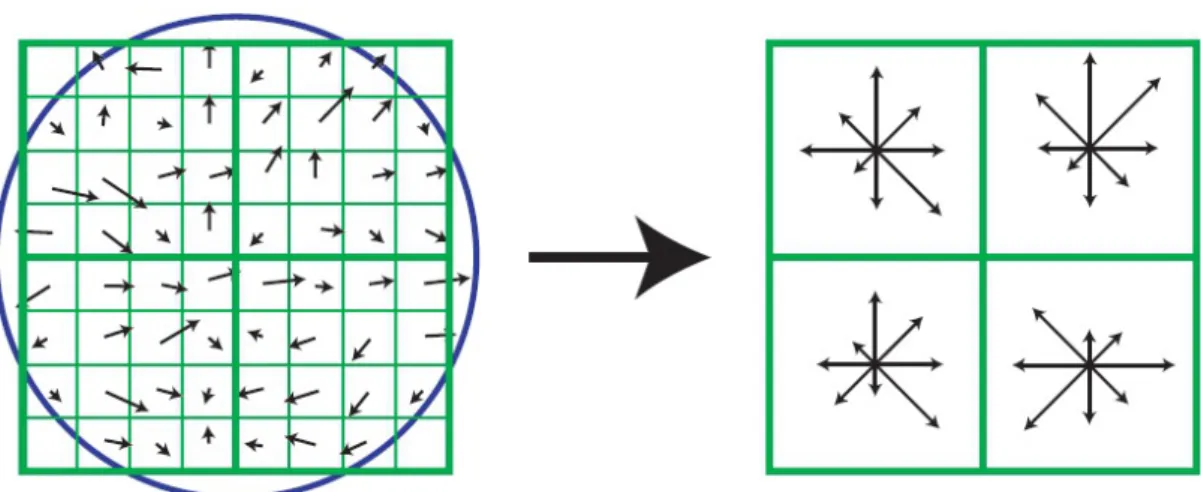
1.1 Demonstration of the results of the diﬀerent tasks developed in the dissertation. In Task 1 the represented local shapes and the matched feature points are shown; inTask 2 the detection result of the improved parametric active contour method is presented and compared to the original algorithm; inTask 3 the extracted urban area and building outlines are marked in red. . . 3 2.1 An octave of L(x, y, σ) images and construction of DoG images. . 12 2.2 Extremum detection: each point is compared with its 26 neighbors

on 3 diﬀerent scales. . . 13 2.3 The original image is on the left, the calculated keypoints with the

assigned orientation can be seen on the right. . . 14 2.4 Keypoint descriptor extraction: The gradient histogram is on the

left, the calculated 128-dimensional descriptor is on the right. . . 15 2.5 Local contour result after the iterative process on diﬀerent frames

for a coherent point: The contour represents the local structure and preserves the main characteristics. . . 17 2.6 Shape description with increasing number of Fourier descriptors . 18 2.7 Characteristic neighborhood and contour . . . 19 2.8 Non-characteristic neighborhood and contour . . . 20 2.9 Keypoint pairs (red/blue) on the video frame, plotted to the ﬁrst

frame while the second moved . . . 22 2.10 Brodatz textures used for training . . . 23 2.11 Brodatz textures used for testing . . . 23

v

(12)

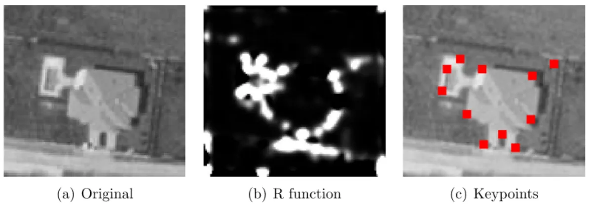
2.12 Simpliﬁed diagram of the workﬂow of change detection process in aerial images. . . 27 2.13 Operation of Harris detector: Corner points are chosen as the local

maxima of the R characteristic function . . . 29 2.14 Original image pairs provided by the Hungarian Institute of Geodesy,

Cartography and Remote Sensing (F ÖMI). . . 30 2.15 Difference maps calculated based on traditional metrics . . . 31 2.16 Logarithmized difference map and result of change keypoint candi-

date detection based on theR-function. Detected change keypoints are marked in red. . . 33 2.17 Remaining change keypoints after ﬁltering with local contour de-

scriptors. . . 34 2.18 Enhanced number of Harris keypoints . . . 35 2.19 Grayscale images generated two diﬀerent ways: (a) is the R com-

ponent of the RGB colorspace, (b) is the u^∗ component of the L^∗u^∗v^∗ colorspace. . . 36 2.20 Result of Canny edge detection on diﬀerent colour components:

(a) is for R component of RGB space; (b) is foru^∗ component of L^∗u^∗v^∗ space. . . 37 2.21 Subgraphs given after matching procedure, edges between con-

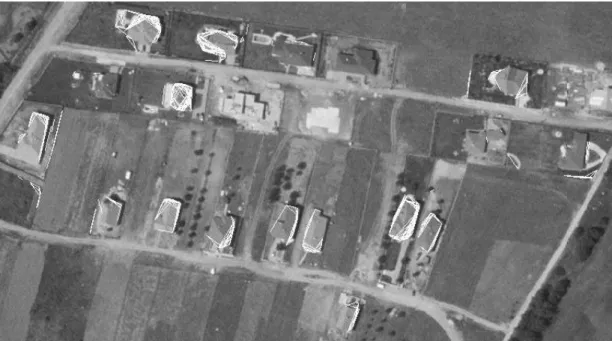
nected keypoints are shown in white. . . 37 2.22 Results of the structural change detection method. Diﬀerent im-

ages shows the result for diﬀerent building outlines for image pair Figure 2.14. . . 38 2.23 Result of the contour detection for aerial image pair provided by

F ¨OMI. . . 39 2.24 Result of the contour detection for aerial image pair provided by

F ¨OMI. . . 40

(13)

3.1 The original f edge map for high curvature boundary: (a) shows the original image, region of interest is in gray; (b) is the f edge map of the marked area. The white rectangle indicates the de- creased f values of the high curvature boundary; (c) is the f_VFC map of the marked area. The white rectangle indicates the de- creased f_VFC values of the high curvature boundary. . . 45 3.2 Eﬀect of Rlogmax characteristic function: (a) is the original im-

age; (b) is the original, f intensity based map of GVF; (c) is the generated and inverted R_logmax characteristic function; (d) is the proposedf_HGVF Harris based map for GVF (Eq. 3.8); (e) shows the generated salient points as the local maxima of the R_logmax function (Fig. 3.2(c)); (f) is the initial contour based on the convex hull of the corner points. . . 47 3.3 Detailed evaluation results. Vertical axis shows the achieved av-

erage F-measure score for each test image separately. Horizontal axis shows the numbered images from the Weizmann database [62]

used for the evaluation set. Separate bars indicate the results of diﬀerent methods: light gray is GVF [20], white is VFC [51], dark gray is HGVF (proposed) and black is HVFC (proposed). . . 50 3.4 Examples of contour detection: The ﬁrst column shows the calcu-

lated initial contour (see Section 3.3.2). Second, third, fourth, ﬁfth and sixth columns present the results for ACWE [47], GVF [20], HGVF (proposed), VFC [51] and HVFC (proposed) methods. . . 52 3.5 Improvement of the diﬀerent feature maps in imageD achieved by

modified Harris based characteristic function: the first row shows the image part with the detected outline, the second row is the corresponding force field and the contour. Columns show the results for GVF [20]; HGVF (proposed); VFC [51] and HVFC (proposed) methods. . . 53 3.6 Comparison with Decoupled Active Contour (DAC) method [52]

with the execution time in brackets. (Image size: 450×297.) . . . 55 3.7 Demonstration of the (a) object rectangle parameters and (b) cal-

culation of the interaction potentials [72]. . . 59

(14)

3.8 Edge and shadow features [8]. . . 60 3.9 Rectangular footprint results, obtained by the MPP based detector

module [72]. . . 62 3.10 Extracted feature points around the object locations estimated by

the MPP based detector. . . 63 3.11 Subgraphs given after matching procedure. . . 64 3.12 Results of the joint building localization and outline extraction

approach. In the ﬁrst column the original images can be seen, the second column shows the detected buildings. . . 65 3.13 (a): Reference image (I_r); (b): Target image (I_t); (c): Probability

map P⁽ⁱ⁾=R_t⁽ⁱ⁾·R⁽ⁱ⁾_d . . . 68 3.14 Steps of the algorithm. 1. Change detection: (a) Change candi-

dates, (b) TheDS_i values for candidates in blue scaled into (0,100) range with ϵ₁ = 3, ϵ₂ = 50 thresholds marked by the red lines, (c) Localization of changes; 2. Lesion boundary recognition: (d) B map, (e) Lesion contour point extraction; (f) The detected lesion boundary. . . 70 3.15 Example for simulated lesions: (a) is the original image without

lesion (red rectangle indicates the location of the lesion in the next images); (b) is the mask of the simulated lesion; (c)–(f) are the images with simulated lesion with 20%, 40%, 60% and 80 % intensity reduction respectively. Image is taken from the MRIcro software. 72 3.16 Reference image, target image and result of detecting appearing

lesions for images provided by MRKK. . . 73 3.17 Sequence diagram of the whole approach. Branches A and B run

in parallel. . . 76 3.18 Contour point detection. (a): Original Harris corner detector [24];

(b): Proposed MHEC point detector; (c)-(d) show the respective objects zoomed. . . 77 3.19 Object separation. (a): Canny edge map; (b): Separated object

contour points marked diﬀerently. . . 79

(15)

3.20 Separation of multiple objects. Flying objects (marked by rectan- gles) are localized based on the separated feature point subsets.

[9] . . . 79 4.1 Simpliﬁed diagram of the workﬂow of urban area detection. . . 83 4.2 Steps of the urban area extraction for the Szada1 image with the

proposed MHEC feature point set. (a) Extracted feature point set. (b) Voting matrix of the referred, non-oriented process [88].

(c) Detected urban area applying the non-oriented process. (d) Detected urban area applying the improved, orientation sensitive process. . . 86 4.3 Detection results for theSzada₅image with diﬀerent voting matrix

formation techniques. (a): Original image. (b): Result of the original, non-oriented method [88] (F-measure value: 0.548). (c):

Result of the proposed orientation sensitive method (F-measure value: 0.717). . . 87 4.4 Ground truth results for Szada₅ image: (a)–(c) images were gen-

erated by three diﬀerent individuals; (d) is the ground truth used for evaluation based on majority voting of previous images. . . 91 4.5 Detection results based for diﬀerent voting matrix techniques. Left:

Original, non-oriented [88]. Right: Proposed orientation sensitive. 93 4.6 Local gradient orientation density (λ_i(φ) function) for the ith fea-

ture point : (a) is the original image denoting the neighborhood of the feature point by a white rectangle; (b) is the cropped image showing the neighborhood of the point; (c) shows the λ_i(φ) function for the feature point, with φ_i =−51. . . 96 4.7 Orientation estimation for a unidirectional image: (a) is the orig-

inal image; (b) shows the feature points in yellow; (c) shows the ϑ(φ) orientation density function of the points in blue, calculated for 15×15 neighborhood. φ ∈ [−90,+90] is the horizontal axis, the number of points is the vertical axis. Theη₂(.) two-component Mixture of Gaussian is in red, detected peaks are θ = −47 and θ_ortho = +53. . . 97

(16)

4.8 Correlating increasing number of bimodal mixture of Gaussians (MGs) with the ϑ orientation density function (marked in blue).

The measured α_q and CP_q parameters are represented for each step. The third component is determined insigniﬁcant, as it covers only 18 MHEC points. Therefore the estimated number of main orientations isq = 2. . . 99 4.9 Orientation based classiﬁcation for q = 2 main orientations with

k-NN algorithm for image 4.8(a): (a) shows the classified MHEC point set, (b)–(d) is the classified image withk = 3,k = 7 andk = 11 parameter values. Different colors show the clusters belonging to the bimodal GMs in figure 4.8(d). . . 100 4.10 Comparing the edge maps for u^∗ channel: (b) shows the result of

the pure Canny edge detection; (c) is the result of the shearlet based edge strengthening. . . 103 4.11 Steps of multidirectional building detection: (a) is the connectivity

map; (b) shows the detected building contours in red; (c) marks the estimated location (center of the outlined area) of the detected buildings. . . 104 4.12 Result of the building detection with one main direction: (a) shows

the detected contours; (b) is the estimated locations of the detected buildings. . . 105 4.13 Qualitative comparison of MPP-based and proposed method: (a) is

the original image part; (b) shows the result of MPP-based method;

(c) is the result of the proposed approach. . . 107

x

(17)

List of Tables

2.1 The number of matches found in the images. Different columns show the different evaluation results: when the real pair was the closest measured LCD and pair was in the five closest LCDs. . . . 21 2.2 Result of texture classification: the number and rate of the correct

classiﬁcations . . . 24 3.1 Average F-measure Score (mean ± standard deviation) for GVF

[20], VFC [51] and the proposed HGVF and HVFC algorithms for 23 images [62]. Bold text indicates the highest achievement. . . . 51 3.2 Performance of diﬀerent active contour algorithms, including ex-

ecution time for images without noise (a) and robustness to increasing Gaussian noise (b) for ACWE [47], GVF [20], HGVF (proposed), VFC [51] and HVFC (proposed) methods. . . 54 3.3 Average SI scores on simulated cases. . . 73 4.1 Average F-measure Score (mean ± standard deviation) for the

evaluated feature point detector methods for Szada dataset. . . . 90 4.2 Quantitative results for Szada dataset . . . 106

xi

(18)

(19)

Chapter 1 Introduction

Automatic detection is a very important task in several computer vision and image understanding applications. Nowadays, with the widespread availability of affordable digital imaging devices and the presence of high capacity personal computers, significance of digital image processing is increasing substantially. As the amount of digital data is huge and manual administration and operation is unmanageable, automatic processing techniques are continuously improved to solve complex challenges in various fields of interest, like video surveillance [42], change detection [43, 81], medical image analysis [76, 77], force protection and defense applications [83], urban area extraction [67, 87] and building detection [89, 74] in aerial images.

As the large variety of applications shows, there is a wide range of tasks to be resolved: different fields have separate concepts and methodology, therefore context-sensitive solutions should be developed to satisfy the special conditions, cope with the altering challenges and reach the exact goals. The aim of this thesis is to present contributions in three main tasks of automatic detection. Although these tasks are related to each other, and the given contributions of different tasks can be fused to be applied for complex solutions, these tasks should be handled separately. The given solutions can all be labeled as techniques for object featuring, but the distinct aims and applications (like extraction, tracking, change detection) need different tools and developments. The short introduction of the three main tasks referred in this thesis:

• Task 1: Giving a low dimensional feature descriptor by exploiting local

1

(20)

structure information around feature points. In this task, the usability of the local shape representation is investigated, where an image series or video is given with a ﬁxed camera position either remaining static or ro- tating during scanning. The local properties are extracted by generating active contour in the small proximity of the feature point, which is then represented by low dimensional Fourier descriptors. The goal is to match feature points through this descriptor set for further post-processing (tracking, classiﬁcation and change detection).

• Task 2: Improving the detection accuracy of parametric active contour algorithms for high curvature, noisy boundaries and giving an automatic initialization technique on single object images. This involves the analysis of the behavior of existing active contour methods and the development of a new feature map which is able to emphasize complex boundary parts and support initialization by deﬁning feature points simultaneously. Moreover, the proposed feature map and point set is adapted successfully for other change detection and multi-object detection applications in registered aerial and medical image series as well.

• Task 3: Detecting built-in areas and building outlines in single airborne images by introducing orientation of the close proximity of the feature points as a novel feature. This task involves the comparison of diﬀerent feature point detectors for built-in area detection, the statistical analysis of extracted

’high-level’ orientation feature to deﬁne main directions of the urban area, and a building detection process applying the given directions for extracting the accurate shape of the buildings without any restrictions (like shape template).

The inputs of all the detailed tasks are digital images and the aim is to perform automatic object detection (outlining) which is then improved to reach the specific goals. Task 1 first outlines the local shape, which is then described by reduced dimensional Fourier descriptors to be compared for different computer vision applications. Besides, the ultimate purpose of Task 2 and 3 is to detect object contours as precisely as possible. Depending on the application, the detected

(21)

Figure 1.1: Demonstration of the results of the diﬀerent tasks developed in the dissertation. In Task 1 the represented local shapes and the matched feature points are shown; in Task 2 the detection result of the improved parametric active contour method is presented and compared to the original algorithm; in Task 3 the extracted urban area and building outlines are marked in red.

(22)

object can vary from a single object (in Task 2) where the point is to recognize the accurate boundary regardless of its complexity, through an appearing Sclerosis Multiplex lesion in a single channel MRI image pair taken by a long time interval to support the radiologist, to an urban area or building in a single airborne image.

Outlining objects is an eﬃcient step in every high-level segmentation process.

It can be considered as a preprocessing step for complex applications. When searching for an object contour, low-level tasks, like edge or line detection could be used as steps of bottom-up processes which are then followed by connection of diﬀerent segments. As the bottom-up approach is a rigidly sequential process, mistakes made at deeper levels are propagated with no chance for correction in higher levels. Therefore, the aim is to use some higher level technique to avoid drawbacks of the sequential method.

Active contour model [17] was introduced for this kind of tasks, using energy minimization as a framework. An energy function is designed by adding suitable energy terms to the minimization, which is able to converge to the desired contour. The model is guided by interactive techniques, developing eﬀective energy functions having local minima in the desired places (on accurate contours) and depending slightly on the starting points.

The novelty of the theory was the management of the contour: handling the whole boundary as a connected system and approximating it in one step, unlike traditional methods performing edge detection ﬁrst and then linking them in a separate step.

In case of the active model, the connected contour system is represented by the well constructed energy terms, which are also responsible for the smoothness of the controlled curve (internal force), for the convergence of the spline towards salient image features like edges, corners (image force) and minimizing the whole energy function to the desired local minimum (external constraint) at the same time. These forces include user interface, automatic attentional mechanisms and high-level interpretation as well.

The eﬃciency of the active contour model relies on the deﬁnition of the energy terms. Therefore, adaptations of the basic model attempt to design such terms, which are able to represents the aforementioned principles. From the given constraints, this dissertation concentrates on the image characteristics and

(23)

tries to improve the image-related energy term. Beside this main concept, it also investigates the signiﬁcance of the local characteristics applied for higher-level purposes.

When designing an eﬃcient function for representing image characteristics, the given function can also be applied for other aims, such as feature point detection.

Due to this advantage, it can also contribute to the initialization process of the active contour model, reducing human interaction.

Moreover, eﬃcient feature maps are constructed with ’higher-level’ information interpretation. By exploiting novel sources, like the connected topology of diﬀerent objects through such channels as their related orientation, accurate object detection task can be raised to even a higher level by invoking an inter-object layer for feature extraction and energy term design.

Regarding the contribution of the thesis in the diﬀerent tasks: Task 1 introduces a low dimensional representation of a converged active contour curve representing the local characteristics of the small neighborhood of a feature point;

Task 2 proposes a novel feature map for the image force term of parametric active contour models; Task 3 investigates the usability of ’higher-level’ feature extraction for eﬃcient object detection.

The outline of the thesis is as follows. Chapters 2 – 4 introduce the contributions of the thesis in Task 1 – 3, by dedicating each chapter to one task.

Chapter 2 concentrates on the challenges of Task 1 and introduces a low dimensional descriptor representing the local characteristics of feature points. Beside describing the novel descriptor, it also investigates the descriptor’s applicability for important computer vision tasks: point matching, texture classiﬁcation and change detection. Chapter 3 presents an improved feature map and initialization approach which can be successfully adapted for parametric active contour method. The introduced method is then extended for other medical and aerial applications for change detection and multi-object detection. Chapter 4 focuses on novel feature extraction for built-in area and building contour detection in airborne images. Finally, a conclusion and the summary of novel scientiﬁc results conclude the dissertation.

(24)

(25)

Chapter 2 Local Contour Descriptors

When searching for an eﬃcient descriptor, the task is twofold: features must describe the featuring patches at a high eﬃciency, while the dimensionality should be kept at a manageable low value.

The main assumption in finding local descriptors is the defect of continuity in the discrete neighborhood or the imperfectness of local shape formats. This chapter investigates the potential applicability of methods in which some formal meaning of the local properties can be represented at a reduced dimension. Curve fitting methods for noisy shapes are called here: active contours. A new local feature descriptor is defined by generating active contours around keypoints. Local contours are characterized by a small number of Fourier descriptors, resulting in a new feature set of low dimensionality. Similarity among keypoints in different images can be searched through these descriptor sets.

2.1 Introduction

Processing databases of video frames is an important task in computer vision, therefore describing local characteristics and registering image keypoints through this descriptor set is necessary. It might be very time consuming if the dimensionality of features is high. An early concept was to ﬁnd speciﬁc keypoints of digital images but nowadays we use much more stable features, so called descriptors, to exploit a considerable amount of usable information from an image area.

Although now we have very eﬃcient local features, we should continuously search

7

(26)

for more applicable solutions. Task is twofold: features must describe the featuring patches at a high eﬃciency, while the dimensionality should be kept at a manageable low value.

Presently used descriptors can be grouped into diﬀerent groups [26]. Distribu- tion based descriptors are using histograms to represent diﬀerent characteristics of appearance or shape. These histograms may based on purely intensity or a combination with distance or gradient distribution, like in scale invariant feature transform (SIFT). Spatial-frequency tehcniques describe frequency content of an image by decomposing the image with Fourier transform into basis functions.

Diﬀerential descriptors computes a set of image derivatives up to a given order for approximating a point neighborhood.

The main assumption in finding local descriptors is to find unique and robust image features for finding and describing image characteristics. However, the dimensionality of these descriptors (e.g. SIFT) is quite large, resulting in time consuming search process for image/video database. A novel local feature detection method [21] proposed an approach for detecting similarity between a template and a given image by using regression kernels, measuring the likeness of a pixel to its neighborhood. The most distinctive features are filtered from this kernel using Principal Component Analysis (PCA). The extracted features are compared with the analogous features of the given image with Canonical Corre- lation Analysis (CCA), followed by a ’resemblance map’ between the two images to produce the probability of similarity. Although this method models a local shape, it is rather interested in detecting a definite template object (e.g. face), and it is not for point pairing.

There are diﬀerent dimension reduction techniques for data of SIFT or similar approaches, like PCA-SIFT [25] or Gradient Location and Orientation Histogram (GLOH) [26]. However, the valid interpretation of data content may be lost during compression. To avoid it, such methods are welcomed, where some formal meaning of the local properties can be maintained at a reduced dimension.

The proposed theory [4] is based on the principle that a saliency point (detected corner etc.) can be considered as a peak/valley concerning the intensity landscape. Diﬀerent feature collection methods scan its neighborhood to describe

(27)

the microstructure somehow. The shape of this peak/valley may also be considered in a contour-map description, but in this low-resolution local neighborhood inside a radius of cc. 5–10 pixels a deﬁnite shape cannot be found. The idea here is to call for curve ﬁtting methods for noisy shapes: active contours. The limited number of pixel values in a local neighborhood is to be surrounded by a curve.

This curve might be distorted due to the transformed image contents, but its main characteristic can remain nearly constant through several frames of videos or through geometrical and illuminational transformations of images from similar scenes.

This chapter is about the possible outcome of a hypothetic approach: can active contour be applied instead or together with other local featuring techniques for a better local description of image content? By examining here the possible solutions, regarding the local features, some measurements and adaptations are also given here about this additional approach.

The crucial step of any local featuring process is to ﬁnd a good salient point.

Several solutions are applied, like Harris [24] corner detection or Difference of Gaussians (DoG) [18], [19] in SIFT. If an efficient approach is used to extract the keypoints, the analytical question should be answered about how to characterize a point’s neighborhood. As the hypothetical discussion only concentrates on this issue, the very efficient SIFT salient point detector is used for localizing the keypoints and giving a good peak/valley definition method as well.

Shape definition around a small salient region (centered by a keypoint) is not easy because of the limited neighborhood in the raw grid-resolution. Conventional shape definition and comparison methods suffer from the limited amount of information around the point. For example, in [23] the dissimilarity between two shapes is computed as a sum of matching errors between corresponding points, together with a term of measuring the magnitude of the aligning transform given by similar shape contents. Edge detection methods, like Canny edge detector [22]

could be adaptable, but as we need a closed curve around the keypoint, active contour method is more eﬃcient as an interpolation-based detector for the given regions.

(28)

2.2 Feature description

The main steps of the proof-of-concept algorithm for extracting local curve characteristics are the following:

1. Localizing keypoints as deﬁned for SIFT [19].

2. Generating Local Contour [20] around the given keypoint.

3. Calculating the Fourier Descriptor [29] for the estimated closed curve.

4. Finding similar curves counting a limited set of components of Fourier De- scriptors [27].

2.2.1 Scale invariant feature transform

Scale Invariant Feature Transform (SIFT) [18, 19] is a 128-dimensional image descriptor, which gives the opportunity for efficient image matching and view invariant visual object recognition, as it is invariant to scale, rotation, illumination and viewpoint. The method first detects interest points, then generates a descriptor of the local image structure by accumulating statistics of local gradient directions of image intensities. The high dimensionality represents large variation, therefore corresponding points can be efficiently matched using this descriptor between different images.

The four main steps of the descriptor extraction are the following:

1. scale-space extrema detection, 2. keypoint localization,

3. orientation assignment, 4. keypoint descriptor.

In the present approach, SIFT method is used only for localizing the keypoints, therefore just the ﬁrst two steps are executed to extract the location of the keypoints. However, in the experimental part SIFT is applied for comparison, thus, the complete algorithm with all the four steps is presented in details.

(29)

2.2.1.1 Scale-space extrema detection

The first stage of the extraction attempts to find ’characteristic scale’ for features, therefore the image is represented by a family of smoothed images known as scale space. The scale space is defined by the function:

L(x, y, σ) = G(x, y, σ)∗I(x, y), (2.1) where∗denotes the convolution operator,I(x, y) is the input image andG(x, y, σ) is the variable-scaled Gaussian:

G(x, y, σ) = 1

2πσ² exp⁻^x2+y

2

2σ2 . (2.2)

Stable keypoint locations of the scale space are then detected by Diﬀerence of Gaussians (DoG) function, where D(x, y, σ) function is given by computing the diﬀerence between two images, one with scale k times by the other:

D(x, y, σ) = (G(x, y, kσ)−G(x, y, σ))∗I(x, y)

=L(x, y, kσ)−L(x, y, σ). (2.3) The L(x, y, σ) convolved images are grouped by octave (an octave corresponds to doubling the value of σ) andk is selected so that a ﬁxed number of convolved images per octave is obtained. DoG images are taken from adjacent Gaussian- blurred images per octave. Figure 2.1 shows the operation of this step. Extrema are then located by scanning each DoG image and identifying local minima and maxima. To detect such locations, each point is compared to its 8 neighbors on the same scale, and 9 neighbors on the higher and lower scale (see Figure 2.2). If the point is the local minimum/maximum of this 26 points, then it is an extremum.

2.2.1.2 Keypoint localization

After extracting extremum points, this step attempts to eliminate points having low contrast or being poorly localized along an edge. For the former case, the scale space value is used. The location of the extremum, ˆx, is determined by taking the derivative of the Taylor expansion (up to the quadratic terms) of the

(30)

Figure 2.1: An octave of L(x, y, σ) images and construction of DoG images [19].

D scale-space function (Eq. 2.3) with respect to x = (x, y, σ)^T and setting it to zero, giving:

ˆ

x=−∂²D

∂x²

−1

∂D

∂x. (2.4)

The function value at the extremumD(ˆx) is investigated and eliminated if|D(ˆx)| is less then 0.03 (assuming image pixel values in the range [0,1]).

For the latter case (eliminating edge responses), observation about principal curvatures can be exploited: an edge point will have large principal curvature across the edge, but a small one in the perpendicular direction. Principal curvatures can be computed from the H Hessian matrix:

H=

[D_xx D_xy D_xy D_yy ]

. (2.5)

Eigenvalues of H (denoted by α₁ and α₂, where α₁ = rα₂) are proportional to the principal curvatures of D. As only the ratio of the eigenvalues is required, not their exact values, motivated by [24], the trace (T r) and determinant (Det) of H is used as follows:

T r(H)²

Det(H) = (α₁+α₂)²

α₁α₂ = (rα₂+α₂)²

rα²₂ = (r+ 1)²

r . (2.6)

If this ratio is over some threshold, the point is taken as an edge point, therefore it is eliminated.

(31)

Figure 2.2: Extremum detection: each point is compared with its 26 neighbors on 3 diﬀerent scales [19].

2.2.1.3 Orientation assignment

After extracting the keypoints, in this step a consistent orientation is assigned to each of them based on local image properties. The keypoint descriptor can later be represented relative to this orientation and achieve invariance to image rotation.

The scale of the keypoint is used to select the related smoothed imageLwith closest scale, therefore all computations are performed scale-invariantly. Magni- tude m(x, y) and orientation θ(x, y) are calculated using pixel diﬀerences:

m(x, y) =√

(L(x+ 1, y)−L(x−1, y))²+ (L(x, y+ 1)−L(x, y−1))², (2.7) θ(x, y) = tan⁻¹

(L(x, y+ 1)−L(x, y−1) L(x+ 1, y)−L(x−1, y)

)

. (2.8)

An orientation histogram with 36-bin is calculated from the gradient orientations of sample points within a region around the keypoint. The highest peak is located and used as the keypoint’s orientation. If more local peaks exist with at least the 80% of height of the highest peak, then the orientation of these peaks

(32)

Figure 2.3: The original image is on the left, the calculated keypoints with the assigned orientation can be seen on the right.

are also assigned to the keypoint, resulting in multiple orientations. This step ensures invariance to image location, scale and rotation.

Figure 2.3 shows the result of orientation assignment. The cyan colored arrows indicate the orientation assigned to each keypoint. The size of the arrow is proportional to the magnitude.

2.2.1.4 Keypoint descriptor

The local gradient data, calculated in the previous step is also used when creating keypoint descriptors. Taking this data, the region of the keypoint is separated into subregions of 4×4 pixel neighborhood and an orientation histogram is calculated with 8 bins for each subregion (see Figure 2.4). This time the gradients are rotated by the previously computed orientation and weighted by a Gaussian function with variance of 1.5 times of the keypoint’s scale. The descriptor is then becomes a vector of all the values of these histograms, resulting in 4×4×8 = 128 dimensions.

Finally the vector is normalized to unit length, ensuring the invariance to aﬃne changes in illumination. For invariance to non-linear changes as well, the vector elements are capped to 0.2 and then the vector is renormalized.

The disadvantage of SIFT is its high dimensionality. However, this eﬃcient data content cannot be compressed [25] without important information loss. Sim- ilar local descriptors [26] also give a batch of collected features. Some of them is

(33)

Figure 2.4: Keypoint descriptor extraction: The gradient histogram is on the left, the calculated 128-dimensional descriptor is on the right.

deﬁned as scale-invariant features, where zoomed attributes describe larger scale connectivity (e.g. scaling in [19]).

2.2.2 Local contour

Instead of the batch of features given by SIFT, here the closed curves around localized keypoints are examined with an algorithm resulting in a meaningful low dimensional descriptor. It is used then for the selection of similar keypoints in diﬀerent images.

The main idea for retrieving further description is analyzing the contour features in the small neighborhood of the keypoint. If signiﬁcant features are extracted, these can be added later to any keypoint descriptor.

Local Contour (LC) is an active contour spline, generated in 11×11 size window with the keypoint in the middle. It is supposed to charactarize the local structure around the keypoint.

Introduced in [17], active contour (AC) is used in computer vision especially for locating object boundaries. The goal of active contour or snake (denoted by x(s) = [x(s), y(s)], s∈[0,1]) is to minimize the following energy:

E =

∫ 1 0

1

2(α|x’(s)|²+β|x”(s)|²) +E_ext(x(s))ds, (2.9)

(34)

whereαandβare weighting parameters for the elasticity and rigidity components of the internal energy; x’(s) and x”(s) are the ﬁrst and second order derivatives with respect to s. The rigidity component is responsible for detecting curvature, setting β = 0 allows the snake to develop a corner. Eext is the external energy derived from the image, representing the image constraints and giving smaller values at features of interest (like edges and ridges), than at homogeneous regions.

The traditional Kass-version had limited utility as the initialization had to be near to the real contour of the object. Problems also occurred when detecting concave boundaries.

To compensate these drawbacks, Gradient Vector Flow (GVF) was a new external force used for snakes [20]. It is computed as a diﬀusion of the gradient vectors of a gray-level or binary edge map derived from the image. The novel E_ext energy is as follows:

E_ext=

∫ ∫

µ(u²_x+u²_y+v_x²+v_y²) +|∇f|²|v− ∇f|²dxdy, (2.10) where the v(x, y) = (u(x, y), v(x, y)) is the GVF ﬁeld that minimizes E_ext, µ is a regularization parameter. The f edge map is derived from the image I(x, y).

One of the generally used forms is:

f(x, y) = |∇(Gσ(x, y)∗I(x, y))|, (2.11) whereG_σis the Gaussian function withσstandard deviation and∇is the gradient operator [20].

The resultant ﬁeld has a large capture range and forces active contours into concave regions. By using GVF, the initial shape of the snake is almost arbitrary.

Although several modiﬁcation have been developed since the publication of GVF method, this approach was applied to test our theory. Therefore, the complete overview of the active contour theory or the operation of other algorithms is not explained here. Further contributions in the active contour ﬁeld along with detailed descriptions are presented in the following chapter.

For initialization, a circle-shaped contour was used, where the center of the circle is the middle of the image and the radius is 3 pixel. After the convergence of the iterative process, the result is supposed to characterize the local structures around the keypoint, see Figure 2.5.

(35)

(a) (b)

Figure 2.5: Local contour result after the iterative process on diﬀerent frames for a coherent point: The contour represents the local structure and preserves the main characteristics.

2.2.3 Dimension reduction and matching with Fourier de- scriptor

The result of the local contour detection is a point series describing the local shape, but the dimension is still high. A dimension reduction technique is needed, which is able to represent the contour efficiently at lower dimension. Fourier descriptors [28] are widely used for shape description, therefore in this step the local contours are represented by the modified Fourier descriptors [29] (MFD) that is invariant to translation, rotation and scaling of shapes. After calculating the low dimensional descriptors, the different images can be matched and compared through these descriptor sets.

The method ﬁrst calculates the discrete Fourier transform (DFT) of this complex shape described by the point sequence, by measuring magnitude values of the DFT coeﬃcients that are invariant to rotation. Denote the m^th pixel of the calculated LC by (x(m), y(m)), then a complex number can be formed as

(36)

Figure 2.6: Shape description with increasing number of Fourier descriptors [30].

z[m] =x[m] +jy[m] the Fourier descriptor is deﬁned as:

F[k] =DF T[z[m]] = 1 L

L−1

∑

m=0

z[m]e⁻^j2πmk/L (k = 0, . . . , L−1), (2.12) where Lis the total number of pixels along the boundary.

If the aim is to reduce the dimension of the local contour descriptor (LCD), the first n < L coefficients F[k] k = 1, . . . , n can be used to represent the local contour. The 0th component of the LCD is discarded to remove the positional sensitivity. The more coefficients used, the more accurate the local contour described (see Figure 2.6). According to the experiments n = 10 was selected to maximize the recognition accuracies, but keeping the dimensionality low.

After having the LCDs for a keypoint, the possibly non-specific LCDs must be filtered out. Similar selection is also applicable in other descriptor methods, like in the keypoint localization step (see Section 2.2.1.2) of SIFT, where low contrasted and poorly localized extremum points are eliminated. The goal is to filter out the points having less characteristic neighborhood.

LCDs can be quite various and distinctive when searching in a large set of keypoints. On the contrary, when characteristic features cannot be found in the neighborhood, the LC remains similar to the initial configuration, therefore many of them can be easily mixed up when close to an average circle-contoured shape (Figure 2.7 and 2.8). Therefore, a prefilter must be used to exclude keypoints with less characteristic LCDs before the pairing process. Thus, aF ilter function is defined to filter out the insignificant curves, which are close to the average meaningless cases:

F ilter(F_f,i,n) ={T h(|Ff,i,1| −Mf,1

V_f,1 ) +...+T h(|Ff,i,n| −Mf,n

V_f,n )}, (2.13)

(37)

(a) Contour in 3D (b) Contour from top view

Figure 2.7: Characteristic neighborhood and contour

where F_f,i denotes the Fourier descriptor of the ith keypoint on frame f, having n coeﬃcients, with F_f,i,1...n denoting the DFT coeﬃcients of the curve, M_f,j and V_f,j are the mean and the variance of the jth component on frame f and T h(.) is a threshold function:

T h(x) =

{ 1 if |x|> t, 0 otherwise.

Choosing t = 1.2, the less signiﬁcant keypoints having F ilter(F_f,i,n) < 3 are eliminated, resulting in a selection of the most representative points, about 30%

of the initial set. The remaining point set with representative LCDs are describing an image, these LCDs have to be compared for image matching.

To compare LCDs for diﬀerent images, symmetric distance computation is introduced and the MFD method has been extended in [27] by proposing the following distance function to compare diﬀerent descriptors:

Dist(F_1,i, F_2,i, n) =σ

(|F1,i,1|

|F_2,i,1|, ...,|F1,i,n|

|F_2,i,n| )

+σ

(|F2,i,1|

|F_1,i,1|, ...,|F2,i,n|

|F_1,i,n| )

, (2.14) where F1,i,1...n and F2,i,1...n denote the DFT coefficients of the compared curves for theith keypoint on different frames, σ is the standard deviation function and n is the threshold, which defines the number of coefficients.

Therefore, a 10-dimensional LCD has been deﬁned, which represents the local characteristics of a keypoint’s neighborhood and a distance function was applied to compare the keypoint descriptors from diﬀerent images.

(38)

(a) Contour in 3D (b) Contour from top view

Figure 2.8: Non-characteristic neighborhood and contour

2.2.4 Experiments

In the following section, the introduced LCDs are evaluated for two, different computer vision tasks. The first is the image matching, where sequential frames of a surveillance video was used, and point matching was performed by comparing the LCDs of the feature points. The second task was the texture classification, where the Brodatz textures were used and LCD method was compared with SIFT method. In this case, 10 training images were selected and the test image was classified after a k-means clustering of the descriptors of the feature points. By comparing the ratio of the points in a given cluster for the training images and the test image, the most similar was selected. As the size of the iterative pattern is varying, dynamic radius was introduced for LC calculation area. An adaptive r value was chosen, based on the variation of FD dimensions.

2.2.4.1 Image matching

Our method was tested on 22 real-life video frames made by an outdoor surveillance camera of a city police central. The algorithm was tested on sequential frame pairs. After extracting the signiﬁcant keypoints, the LCDs are compared, the distance between them is measured by Equation 2.12. To evaluate results, the ground truth data of matching keypoint pairs can be deﬁned by tracking or SIFT keypoint matching algorithm. Let p_1,i denote the ith keypoint on Frame 1

(39)

Frame pairs Nr. of pointpairs Real pair is closest(%) Real pair in 5 closest(%)

1-2 10 6 (60%) 8 (80%)

8-9 20 8 (40%) 14 (70%)

18-19 22 7 (32%) 16 (73%)

Table 2.1: The number of matches found in the images. Different columns show the different evaluation results: when the real pair was the closest measured LCD and pair was in the five closest LCDs.

and p_2,j its pair on Frame 2, K is the number of signiﬁcant keypoints on Frame 2. The results were evaluated in two ways:

• The real pair for p_1,i is the closest LCD:

j = argmin

k∈[1,...,K]

(Dist(F_1,i, F_2,k,n))

• The real pair is in the ﬁve closest LCDs.

As it can be seen in Table 2.1 the real pair was the best match approximately in the 40% of the cases (altogether in 21 out of the 52 cases), and in 73% of the pairs it was in the best ﬁve matches. A typical result is on Figure 2.9, where the detected keypoint pairs are shown on one frame. The original keypoint is in red, and its tracked (closest) pair is in blue.

2.2.4.2 Texture classiﬁcation

The above results showed that LCDs can be comparable features against compressed descriptors. So, due to the promising result for image matching, the method was tested in another challenging ﬁeld of image segmentation, the texture classiﬁcation.

A well-known and widely-used dataset for texture classification is the Brodatz- textures, which consists of 112 different natural textures, like brickwall, grass, etc. This dataset was used to compare the SIFT method and the proposed LCD method for classifying textures. The major steps of the classification algorithm are the following:

1. Generating the descriptors (either SIFT or LC) for training and test images.

(40)

Figure 2.9: Keypoint pairs (red/blue) on the video frame, plotted to the ﬁrst frame while the second moved

2. Clustering the descriptors of all images with k-means algorithm.

3. Classifying the test image according to the clustering results.

Both for SIFT and LCD, 10 diﬀerent images for training and 5 images for testing were chosen. These images can be seen in Figure 2.10 and 2.11. In one iteration, all the 10 training images and one test image was used for comparison and classiﬁcation.

The ﬁrst step, in case of SIFT, was to generate the 128-long SIFT descriptors (Section 2.2.1). While in case of LCDs, the ﬁrst three steps, mentioned in the beginning of Section 2.2, were executed.

The second step was the clustering, where k-means algorithm, withk = 15 was used. The clustered results were summarized and normalized. Therefore, every image had a value for every cluster, which meant the ratio of the descriptors clas- siﬁed into the actual cluster, resulting in a descriptor set: {R(i,1), . . . , R(i, k)}

(41)

(a) 1 (b) 2 (c) 3 (d) 4 (e) 5

(f) 6 (g) 7 (h) 8 (i) 9 (j) 10

Figure 2.10: Brodatz textures used for training

(a) 1 (b) 2 (c) 3 (d) 4 (e) 5

Figure 2.11: Brodatz textures used for testing

describing the distribution, where i is the image and k is the number of the clusters.

The last step was to compare the {R(i, .)} descriptor set and classify the test image. The classiﬁcation was based on the normalized results of the clustering.

For each training image the R(i, j) cluster ratio values were compared with the test image and the difference was summarized. In Equation 2.15, Diff(tr, te, j) means the difference of training imagetr, test imagetefor the clusterj. Therefore the total difference:

Diﬀ(tr, te) =

∑k j=1

Diﬀ(tr, te, j) =

∑k j=1

|R(tr, j)−R(te, j)| (2.15) After counting the diﬀerence for all training images, the lower value means the higher similarity.

(42)

Test image Pair SIFT LCD with SR(r=20) LCD with DR(r)

1 2 4 (80%) 4 (80%) 5 (100%) (20)

2 2 5 (100%) 4 (80%) 4 (80%) (20)

3 3 5 (100%) 5 (100%) 5 (100%) (20)

4 6 0 (0%) 0 (0%) 5 (100%) (25)

5 10 5 (100%) 0 (0%) 5 (100%) (30)

Table 2.2: Result of texture classiﬁcation: the number and rate of the correct classiﬁcations

Results of classification iterations can be seen in Table 2.2. Every test image was classified 5 times. The number of correct classifications are summarized in the table for each case. The number of the most similar pair (used as ground truth) from the training images is also indicated. The third column contains the classification results for the SIFT method.

The fourth column represents the results of the LCD method, where LCDs generated in a static 20×20-size neighborhood of the keypoint (called as static radius (SR)). The 4th and 5th test images showed poor results. In these two cases the iterative pattern is larger, than 20×20, so the fixed, r = 20 radius is too small and should be extended. To solve this problem, dynamic radius (DR) was introduced. DR is counted based on the variation of the FDs. To test this variation, LC and then FD is calculated (see Eq. 2.9 and 2.12) in the r×r neighborhood around the feature point. If the iterative pattern is large, extending the radius results in the variance of the main FD components. This means, the contour of the pattern is more characteristic. Similarly, if the iterative pattern is small, extending the radius has no effect on the FDs, as the contour of the pattern remains nearly constant. Therefore, the radius should be extended until the variance of the main FD components is not exceeding a threshold and remaining quasi-constant. The last column shows the results of the LCD method with DR. By using the DR, results for the 4th and 5th test images are improving significantly. The calculated DR is also represented for each case.

(43)

2.3 Detection of structural changes in long time-span aerial image samples

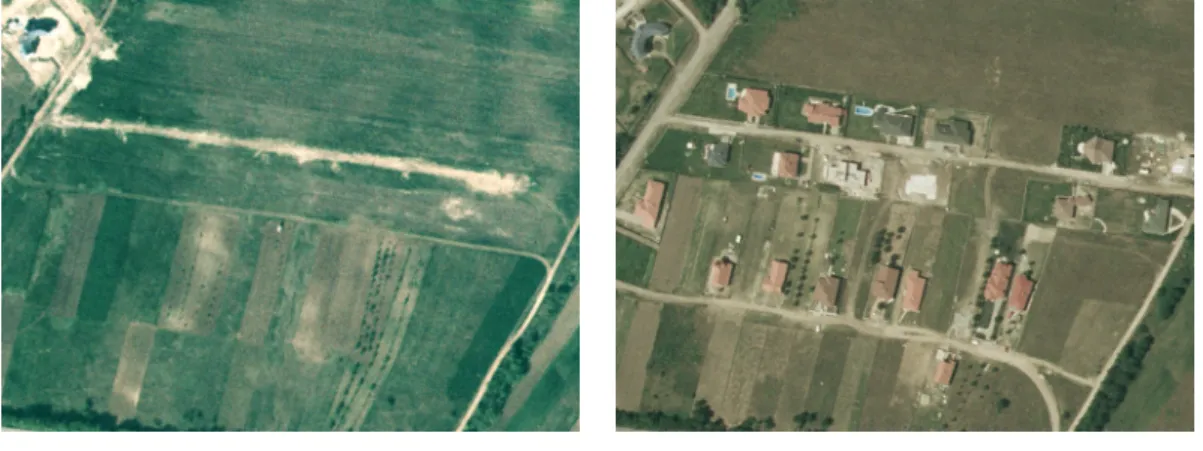
This section presents an application of local contour descriptors (introduced in the previous section) to find changes in remote sensing image series [6]. Some remotely sensed areas are scanned frequently to spot relevant changes, and several repositories contain multi-temporal image samples from the same area. The proposed method finds changes in images scanned by a long time interval in very different lighting and surface conditions. The presented method is basically an ex- ploitation of Harris saliency function and its derivatives for finding feature points among image samples. In the first step, the Harris corner detection is introduced for difference extraction and localization of change keypoint candidates, instead of the simple edge functions. Change keypoints are then filtered based on local contour descriptors, by comparing the changes in the neighborhood between the older and newer image. The boundary hull of changing objects is estimated by fusing the connectivity information and the change keypoint set with a graph- inspired technique. The method is evaluated on registered remote sensing image pairs taken in 2000 and 2005, therefore having different color and illumination features.

2.3.1 Motivation and related works

Automatic evaluation of aerial photograph repositories is an important ﬁeld of research since manual administration is time consuming and cumbersome. Long time-span surveillance or recognition about the same area can be crucial for quick and up-to-date content retrieval. The automatic extraction of changes may fa- cilitate applications like urban development analysis, disaster protection, agri- cultural monitoring, and detection of illegal garbage heaps, or wood cuttings.

The obtained change map should provide useful information about size, shape, or quantity of the changed areas, which could be applied directly by higher level object analyzer modules [31], [32]. While numerous state-of-the art approaches in remote sensing deal with multispectral [33], [34], [35], [36] or synthetic aperture radar (SAR) [37], [38] imagery, the signiﬁcance of handling optical photographs is also increasing [39]. Here, the processing methods should consider that several

(44)

optical image collections include partially archive data, where the photographs are either grayscale or contain only poor color information. This section focuses on finding contours of newly appearing/fading out objects in optical aerial images which were taken with several years time differences, in different seasons and in different lighting conditions. In this case, simple techniques like thresholding the difference image [41] or background modeling [42] cannot be adapted efficiently since details are not comparable.

In the literature one main group of approaches is the postclassification comparison, which segments the input images with different land-cover classes, like woodlands, barren lands, and artificial structures [43], obtaining the changes indi- rectly as regions with different classes in the two image layers [39]. The proposed approach follows another methodology, like direct methods [33], [35], [37], where a similarity-feature map from the input photographs (e.g. a difference image) is derived, then the feature map is separated into changed and unchanged areas.

This direct method does not use any land-cover class models, and attempts to detect changes which can be discriminated by low-level features. However, this approach is not a pixel-neighborhood maximum a priori probability system as in [40], but a connection system of nearby saliency points. These saliency points deﬁne connectivity relations by using local graphs for estimating the outline of the objects. Considering this estimated polygon as a starting spline, the method searches for object boundaries by active contour iterations (See Figure 2.12).

The main saliency detector is calculated as a distinguishing metric between the functions of the different layers to extract saliency point set. Harris detector is proved to be an appropriate function for finding the dissimilarities among different layers and handling the varying illuminational circumstances, when comparison of other low-level features is not possible because of the different lighting, color and contrast conditions.

Local structure around keypoints is investigated by local contour descriptors (see Section 2.2.3), representing the local microstructure around keypoints. How- ever, the local contour is generated by edginess in the cost function (gradient information in the external energy), while keypoints of junctions (corners) are characterized in the localization step. To ﬁt together the deﬁnition of keypoints and their active contour around them, Harris corner detection was applied as an

(45)

Figure 2.12: Simpliﬁed diagram of the workﬂow of change detection process in aerial images.

outline detector instead of the simple edge functions. This change resulted in a much better characterization of the local structure.

2.3.2 Change detection with Harris keypoints

In case of long time-span aerial image pairs, many changes might have happened during the elapsed time between the scanning of images. Therefore, the image content might have changed signiﬁcantly. Moreover, the altering weather conditions (diﬀerent illumination angle, season, etc.) cause varying color, contrast and

(46)

shadow information. Due to these diﬀerences, SIFT cannot be used for image matching and keypoint localization, unlike in Section 2.2.1.2.

When localizing changes, a robust method is needed which is able to cope with the varying illumination and emphasize the structural changes at the same time. As the available aerial image pairs are already registered manually by the Hungarian Institute of Geodesy, Cartography and Remote Sensing (F ¨OMI), the idea was to generate a diﬀerence image based on some metric, emphasizing changes between images. The applied metric was the Harris corner detector’s characteristic function [24], which is proved to be fairly invariant to illumination variation and image noise, moreover the detector itself is reliable and invariant to rotation [44].

2.3.2.1 Harris corner detector

The Harris detector [24] is based on the principle that at corner points intensity values change largely in multiple directions. Change D for a small (x, y) shift is given by the following Taylor expansion:

D(x, y) = Ax²+ 2Cxy+By², (2.16) which can be rewritten as

D(x, y) = (x, y)M(x, y)^T. (2.17) Here, M is the Harris matrix:

M =

[ A C

C B

]

, (2.18)

where A = ˙x² ∗w, B = ˙y² ∗w, C = ˙xy˙ ∗w. ˙x = ^∂I_∂x and ˙y = ^∂I_∂y denote the approximation of the ﬁrst order derivatives of the I image, ∗ is a convolution operator and w is a Gaussian window.

The curvature behavior around an image point can be well described by the Taylor expansion (Eq. 2.16). When D is reformulated by a structure tensor (Eq. 2.17) and becomes closely related to the local autocorrelation function, M describes the shape at the image point. The eigenvalues of M will be proportional to the principal curvatures of the local autocorrelation function and form a