Event based diagnosis of process systems
PhD Thesis
Author: Attila T´ oth
Supervisor: Katalin M. Hangos, DSc.
University of Pannonia
Faculty of Information Technology
Doctoral School of Information Science and Technology 2016
EVENT BASED DIAGNOSIS OF PROCESS SYSTEMS
Értekezés doktori (PhD) fokozat elérése érdekében
Írta:
Tóth Attila
Készült a Pannon Egyetem Doktori Iskolájának keretében
Témavezetők: Dr. Hangos Katalin
Elfogadásra javaslom (igen / nem) ………..
(aláírás) A jelölt a doktori szigorlaton ……….%-ot ért el.
………..
(aláírás) Az értekezést bírálóként elfogadásra javaslom:
Bíráló neve: ……… igen / nem
………..
(aláírás)
Bíráló neve: ……… igen / nem
………..
(aláírás)
Veszprém,………. ………..
a Bíráló Bizottság Elnöke
A doktori (PhD) oklevél minősítése:
………..
Contents
Acknowledgments 7
Abstract 10
1 Introduction 15
1.1 Motivation . . . 15
1.2 Review of discrete methods applied in process systems . . . . 15
1.2.1 Diagnostic methods based on hazard identification in- formation . . . 16
1.2.2 Diagnostic methods based on clustering and statistics . 17 1.2.3 Approaches to diagnostic decomposition . . . 18
1.3 Problem statement . . . 19
1.3.1 Related common taxonomy . . . 20
1.4 Thesis structure . . . 21
2 Basic notions 23 2.1 System model . . . 23
2.2 The diagnostics task . . . 24
2.3 Inputs and outputs, qualitative range space . . . 25
2.4 Events . . . 25
2.5 Traces . . . 26
2.6 Faults . . . 28
2.7 A simple composite process system . . . 29
2.7.1 Nominal trace . . . 30
2.7.2 Faults . . . 30
2.8 Summary . . . 33
3 P-HAZID diagnostics 35 3.1 Introduction . . . 35
3.2 Basic notions . . . 36
3.2.1 Flattening of traces . . . 37
3.2.2 Deviations . . . 37
3.2.3 P-HAZID table . . . 39
3.3 P-HAZID based diagnostics . . . 41
3.3.1 Additional assumptions . . . 42
3.3.2 Algorithm description . . . 42
3.3.3 Analogy with if-then rules . . . 44
3.4 Diagnostics case study . . . 44
3.4.1 Flattening of the traces . . . 45
3.4.2 Acquiring deviations from faulty traces . . . 45
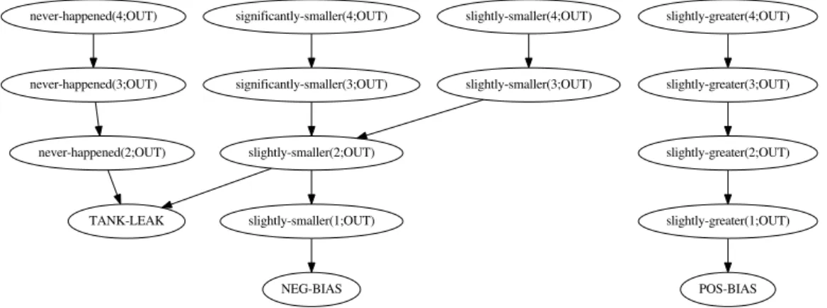
3.4.3 Reasoning graphs . . . 46
3.4.4 P-HAZID table . . . 47
3.4.5 Execution of the algorithm . . . 47
3.4.6 Observations . . . 50
3.5 Summary . . . 51
4 Diagnostics using clustering 53 4.1 Introduction . . . 53
4.2 Basic notions . . . 54
4.2.1 Mapping of qualitative values to real ones . . . 54
4.2.2 Coordinate-vectors of events and traces . . . 56
4.2.3 Event and trace distances . . . 57
4.3 The diagnostic method . . . 58
4.3.1 Additional assumptions . . . 59
4.3.2 Clustering of traces . . . 59
4.3.3 Steps of the Diagnostic Procedure . . . 61
4.3.4 Dealing with faults not considered a priori in the train- ing set . . . 62
4.3.5 Trace coordinates with different measurement units . . 62
4.3.6 Limitation on the lengths of traces . . . 63
4.4 A diagnostic case study . . . 63
4.4.1 Measurement errors . . . 64
4.4.2 Description of the case study . . . 65
4.4.3 Execution of the algorithm . . . 65
4.4.4 Effect of different mapping functions . . . 69
4.4.5 Observations . . . 71
4.5 Summary . . . 72
5 Decomposition in event-based diagnostics 75 5.1 Introduction . . . 76
5.2 Components, component structure and trace decomposition . . 76
5.2.1 Component . . . 77
5.2.2 Component graph and component path . . . 77
5.2.3 Start condition . . . 79
5.2.4 Component mapping function . . . 79
5.2.5 Trace fragments . . . 80
5.3 Component based diagnostics . . . 81
5.3.1 Additional assumptions . . . 81
5.3.2 General algorithm . . . 82
5.4 A diagnostics case study . . . 84
5.4.1 Determining the component graph . . . 84
5.4.2 Nominal and faulty traces for components . . . 85
5.4.3 Component based P-HAZID diagnoser . . . 85
5.4.4 Component based Clustering diagnoser . . . 85
5.4.5 Observations . . . 88
5.5 Summary . . . 90
6 Conclusion 91 6.1 Theses . . . 91
6.1.1 Thesis 1 - the P-HAZID diagnoser (Chapter 3) . . . 91
6.1.2 Thesis 2 - the Clustering diagnoser (Chapter 4) . . . . 92
6.1.3 Thesis 3 - decomposition method for event-based diag- nostics (Chapter 5) . . . 93
6.2 Own publications supporting the thesis points . . . 93
6.3 Further research directions . . . 94
6.3.1 On-line diagnostics . . . 94
6.3.2 Improving robustness during clustering . . . 95
6.3.3 Validation of P-HAZID tables . . . 95
6.3.4 Further application in real process systems . . . 95
6.3.5 Unifying the P-HAZID and the Clustering diagnoser . 96 7 Appendix 97 7.1 The P-HAZID reasoning method . . . 97
7.2 Realistic use-case for the Clustering diagnoser . . . 100
7.2.1 Tennessee-Eastman process . . . 101
7.2.2 Preparation of the data . . . 102
7.2.3 Results . . . 103
7.2.4 Observations based on the results . . . 106
Bibliography 109
Acknowledgments
First and foremost I would like to thank my supervisor, Professor Katalin M. Hangos for her endless support and motivation during my PhD studies.
I could not have been able to get this far without all the guidance she gave to me during these years.
I would also like to thank my wife for supporting me during all the long evenings and weekends when I was way too busy doing the lengthy work of the research. I will always remember all the kind words you have said when the end of this very long journey seemed too distant.
Last but not least, I would like to thank my parents for all their support and encouragement during all of my school and university years. Without them it would not have been possible for me to pursue a study of this level, which I always wanted. Specifically, I would like to thank my father for introducing me to the fascinating world of computer science.
Abstract
In order to prevent or mitigate losses caused by plant faults, early and ac- curate fault diagnostics during the operation of modern day process systems is a very important task. In this dissertation a few diagnostics methods for complex composite process systems controlled by operational procedures are presented.
First a methodology for capturing expertise about the execution process system operational procedures in the form of specifically constructed spread- sheets (P-HAZID tables) is described. Experts of the process system can use this methodology to create a fault model and store diagnostics related knowledge about the system. A reasoning algorithm is proposed, which can perform fault diagnosis based on this model and the actual dynamics of the plant. This method is similar to the widely known if-then rules from rule- based expert systems in artificial intelligence but extends it with the ability to reason about differences between event sequences.
A solely observation-based diagnostic approach which can work on obser- vations of nominal and faulty modes of a process system is also proposed.
The model of this diagnostic method uses a popular machine-learning tech- nique called clustering. The algorithm suggests fault modes for the current operational procedure of the process system based on historical operational procedure logs gathered from past runs of the operational procedure under different faulty conditions.
One can see value in decomposing these diagnostic ideas to enable their use in more complex process systems and diagnostic problems. Therefore a diagnostic decomposition approach is proposed which can be used to scale up standalone diagnostic methods by bringing the diagnostics down to the level of the components from the level of the system.
El˝ osz´ o
A korai ´es pontos hibadiagnosztik´anak nagy szerepe van napjaink bonyolult folyamatrendszereinek ¨uzemeltet´ese sor´an, annak ´erdek´eben hogy az esetleges meghib´asod´asok ´altal okozott vesztes´eget elker¨ulj¨uk vagy cs¨okkents¨uk. Ebben a disszert´aci´oban p´ar ´ujszer˝u diagnosztikai m´odszer ker¨ul ismertet´esre, amit oper´atori elj´ar´asok ´altal vez´erelt folyamatrendszerek hibadiagnosztik´aj´ara lehet felhaszn´alni.
Els˝o k¨orben egy olyan m´odszer ker¨ul ismertet´esre, amivel a folyama- trendszer szak´ert˝oi ¨uzemeltet´esi tud´asukat speci´alis t´abl´azatok (P-HAZID t´abl´azatok) form´aj´aban tudj´ak r¨ogz´ıteni. ´Igy lehet˝os´eg¨uk ny´ılik arra is hogy diagnosztikai ismereteket ´es a hib´as m˝uk¨od´es modelljek´ent t´abl´azatos form´a- ban elt´arolj´ak. Egy k¨ovetkeztet´esi algoritmus is ismertet´esre ker¨ul, ami k´epes hibadiagnosztik´at v´egrehajtani ezen t´abl´azat ´es a folyamatrendszer m˝uk¨od´ese alapj´an. Ez a m´odszer a sz´elesk¨orben ismert ha-akkor szab´alyokon alapul, kieg´esz´ıtve azt az esem´enysorozatokra vonatkoz´o k¨ovetkeztet´es k´epess´eg´evel.
Egy puszt´an megfigyel´es-alap´u diagnosztikai m´odszer is ismertet´esre ker¨ul, ami a folyamatrendszer norm´alis ´es hib´as megfigyelt m˝uk¨od´esi m´odjai alapj´an m˝uk¨odik. Ennek alapja egy n´epszer˝u g´epi tanul´asi megk¨ozel´ıt´es, a csopor- tos´ıt´as (clustering). Ennek sor´an a kor´abban felv´etelre ker¨ult norm´alis ´es hib´as m˝uk¨od´esi m´odok ¨osszehasonl´ıt´asra ker¨ulnek az aktu´alis m˝uk¨od´essel, ez alapj´an javasol a m´odszer lehets´eges meghib´asod´asokat.
Mivel nagy rendszerek ´es bonyolult diagnosztikai probl´em´ak eset´en a fel- haszn´alt m´odszereket ´erdemes dekompon´alni, ez´ert egy dekompoz´ıci´os meg- k¨ozel´ıt´es is ismertet´esre ker¨ul a disszert´aci´o v´eg´en. Ennek seg´ıts´eg´evel egy nagyobb rendszerszint˝u diagnosztikai m´odszer t¨obb kisebb, egyszer˝ubb kom- ponensszint˝u m´odszer ¨osszet´etel´ev´e alak´ıthat´o ´at.
Zusammenfassung
Heute die fr¨uhe und genaue Fehlerdiagnose spielt eine große Rolle in den Be- trieb von komplexen Prozesssysteme, um die potenzielle, durch den Ausfall verursachten Verluste zu vermeiden oder zu reduzieren. In dieser Arbeit wird ein paar neue diagnostische Verfahren beschrieben, die f¨ur die Fehlerdiag- nose von Operatorsverfahren gesteuerte Prozesssysteme verwendet werden k¨onnen.
In der ersten Runde wird so ein Verfahren beschrieben, wobei die Ex- pertenwissen ¨uber Betriebsbereich in Form von speziellen Tabellen (P-HAZID Tabellen) aufgezeichnet werden k¨onnen. Auf dieser Weise werden wir die Gelegenheit haben die Fehlermodel zu erzeugen und die Diagnostikerfahrun- gen ¨uber das System zu speichern. Es wird auch eine Algorithmus dargelegt, welche f¨ahig ist mit der Hilfe der P-HAZID Tabellen und der Prozesssys- teme eine Fehlerdiagnose auszuf¨uhren. Dieses Verfahren ist weit bekannt und basiert auf den Regeln ”Wenn-Dann”. Dieses erg¨anzt den Regeln mit der F¨ahigkeit der Schlussfolgerung.
Eine bloße Beobachtung basierte Diagnoseverfahren ist ebenfalls vorge- sehen, die auf der Grundlage der beobachteten normalen und fehlerhaften Betrieb des Prozesssystems arbeitet. Es basiert auf einem popul¨aren Maschi- nenlernansatz, auf der Gruppierung (Clustering). So die zuvor aufgezeich- neten normalen und fehlerhaften Betriebsarten werden mit den aktuellen Be- trieb vergleicht. Anhand die Ergebnisse der Vergleichungen wird Vorschlage
¨
uber die Defekte gegeben.
Es wird auch eine Zersetzungsann¨aherung beschrieben, da es lohnt sich die verwendeten Methoden auseinander nehmen bei den großen Systemen und komplizierten Problemen. Aus mehreren, kleineren und einfacheren kompo- nentenebene Methode kann eine gr¨oßere Systemebene Methode aufgebaut werden.
Chapter 1 Introduction
1.1 Motivation
Early and accurate fault diagnostics is one of the most important challenges during the operation of modern day process systems. Primeval fault mitiga- tion and isolation due to proper diagnostics plays a crucial role in avoiding huge losses and plant breakdowns caused by the consequences of initially smaller and isolated but propagating failures discovered too late. The ap- plication of an intelligent fault diagnostics solution for a plant might lead to safer and less complicated operation with decreased operational costs, and leaves less possibilities for human errors.
The importance of the field is indubitable, on the other hand, creating a proper diagnostic solution is not an easy task. Many aspects of the plant need to be taken into account and there is no general solution which fits all scenarios. Numerous diagnostic solutions are available in the literature, ranging from simple techniques (for instance, simple logics in the controller of the system) to very complex ones (such as rule based expert systems).
The motivation of this work is to contribute a few novel event-based qualitative diagnostics methods to this field of study.
1.2 Review of discrete methods applied in process systems
Because of its vital importance, the literature of discrete diagnostic ap- proaches is enormously wide, with the model-based methods for fault de- tection and isolation are the most widespread.
1.2.1 Diagnostic methods based on hazard identifica- tion information
Depending on the a priori and measured information that is available for diagnostics, the fault diagnostic approaches for process systems are cate- gorized into quantitative, qualitative and process history based approaches in [51]. Model-based qualitative diagnostic approaches apply approximate
”qualitative” information for both the models and the measured signatures or symptoms.
Process fault diagnostics based on process and fault models had been widely described by Venkatasubramanian in review articles [49], [48] and [50].
According to [48], model based a priori knowledge can be broadly classified as quantitative and qualitative. Fault detection using these qualitative models can be performed by using expert systems with different kind of reasoning, using signed directed graphs (SDGs) for modeling cause-effect relations (for instance in [47]) or fault trees describing the relations between primary events to top level events or hazards. Fault propagation analysis [21] can be used for the identification of faults, causes and consequences in a systematic manner.
In the last review article of the series by Venkatasubramanian on process systems diagnostics ([50]), process history based methods are surveyed. In- stead of an apriori model, these methods require a large amount of historical process data, and they can be classified by the way they extract information from the process data (this operation is called feature extraction). Feature extraction can be qualitative (for example using rule-based expert systems or qualitative trend analysis) and quantitative (using statistical methods, such as PCA or neural networks).
Hazard identification (HAZID, see [16]) has been long taken as an inde- pendent activity from diagnostics, but the information they built on has a lot of common elements. The HAZOP (Hazard and Operability, see [5], [15], [26]) and FMEA (Failure Effect and Mode Analysis, see [6]) are two funda- mentally different analysis methods for hazard identification, where HAZOP is deviation-driven and FMEA is process component-driven. Due to the com- plexity of real process systems, the time-consuming and error-prone manual construction of HAZOP and FMEA tables has been identified as a major bot- tleneck in hazard identification of process systems. Fortunately, there have been results for automated generation of them (in the previously mentioned review articles and for HAZOP, in [51] together with a concrete application in [49]). Another possible way is to use qualitative models in such an anal- ysis (again, for HAZOP, see [10] with a batch process system application in [36]). An attempt to unite the two different diagnostic information stored in HAZOP and FMEA analysis results, called the blended HAZID methodol-
ogy was described in [42] together with its use for process system diagnostics tasks.
The blended HAZID approach (described thoroughly in [42]) combines the system-driven HAZOP and the component-driven FMEA into one method- ology, attempting to minimize their weaknesses and utilize their strengths at the same time. Unlike the original HAZOP and FMEA, three main steps in the initial analysis are needed (based on [42]):
1. Decompose the system into subsystems - the analysis is done in sub- system level onwards.
2. Find deviations from intended functions, with their causes and impli- cations.
3. Elicit the causes and effects of each fault per component in every sub- system on the function of the system.
As a result of the analysis, a cause-implication directed graph (see [34] for an example) can be drawn for each identified failure to visualize casual re- lationships between failures and components. The nodes in this graph are either components or functional failures and each edge represents a causal relationship between them. This graph is a powerful visualization tool for plant operators.
For describing arbitrary output signal values qualitative trend analysis (QTA) can be used, by comparing qualitative trends of nominal and actual signal values (a good example can be found in [30]). In some newer results (in [31]), these methods have been even combined to perform fault diagnostics.
1.2.2 Diagnostic methods based on clustering and statis- tics
As a technique used thoroughly in machine learning, clustering is used in systems for process diagnostics. For instance, as a popular method in the field, the k-means clustering algorithm (refer to [3]) is used for process sys- tem modeling in [17]. Different other approaches are using the fuzzy c-means clustering (FCM, described in [2]), a method based on the concept of fuzzy sets and logic (described originally in [28]). For example fuzzy c-means clus- tering for fault classification is reported in [32] and [37] while it is used for process control in [25].
A special type of historical process data are the so called alarms, the timed sequence of which has been utilized for early fault detection and diag- nostics in [1]. These alarm sequences can be thought as event logs. In [46] a
process mining tool called ProM is described which is capable of discovering process models in the form of Petri Nets, using event logs collected from pro- cess systems. This tool supports conformance checking, verification, model extension and transformation as well as model discovery. A ProM extension described in [17] uses k-means clustering for categorizing event logs prior to mining them, in order to achieve faster operation. In a slightly different ap- proach described in [40], Petri nets are used to build up models from event sequences, and the fitness and appropriateness of the model is calculated.
The most widely used quantitative feature extraction procedures use sta- tistical methods (e.g. PCA or PLS) for process monitoring and fault detec- tion, for which good review papers have appeared recently, see [54], [38] or [24]. A recent improvement of the PLS method capable of detecting small faults have been reported in [23]. However, these methods usually assume steady-state operation condition of the system to be diagnosed, and fail dur- ing transient operations.
1.2.3 Approaches to diagnostic decomposition
The concept of decomposing a problem into related subproblems is used widely in mathematics and computer science in order to solve bigger prob- lems by combining the solutions for their smaller subproblems. This idea had been generalized for process system diagnostics as well in numerous cases in the past. Process systems are mostly built from similar components, there- fore by decomposing them, and diagnosing the components one by one might be more effective than diagnosing the whole system at once. As described in [41] artificial intelligence based searching techniques (such as constraint satisfaction search) fall into the set of NP-hard problems (see [29]). A subset of fault diagnostics approaches uses these techniques, therefore the idea of decomposition is used at a few related works already in the field of process system diagnostics (such as the previously mentioned BL-HAZID methodol- ogy) to cope with the problem of NP-hardness.
The original HAZID method (on which the BL-HAZID approach is based on, see [5]) provides a systematic process in which it breaks down the process system into separately manageable sub-components for collecting hazards of the system. Various hazards are collected separately for the sub-components by the HAZID team performing the study, making their task less complex.
A distributed on-line diagnostics framework is proposed in a recent article [19] for fault detection, isolation and identification. This diagnostic approach scales better than the traditional centralized approaches for model-based di- agnostics and it uses an extension of the Possible Conflicts (PC) decomposi- tion technique (see [33]). The PC decomposition technique originally requires
the use of a central coordinator, but in this extended case the diagnostics is performed by independent distributed diagnosers which do not need any coordination over or communication between them.
Qualitative physics is used for process system modeling as a common sense reasoning about physical systems. This approach is based on qualitative or ordinary differential equations describing the process system to be diagnosed.
These qualitative dynamic models together with many different methods use an abstract hierarchy of process knowledge which is based on decomposing the process system into subcomponents, in order to decrease computational complexity and speed up the diagnostics task.
A process system structural decomposition method for performing diag- nosis based on qualitative physics is described in [21], where the the physical connections and fault propagation through them is emphasized. Apart from this, the article describes an object-oriented process system topology model- ing approach with which the component-specific fault model can be shared between components of the system.
The laws of qualitative physics can be described using the concept of qualitative reasoning. This technique attempts to cover physical laws of the system as qualitative rules instead of ordinary differential equations (which can be considered as quantitative). In that way it is closer how the human mind model and reason about the behavior of a system than differential equations. Refer to [43] for a detailed description of this methodology.
1.3 Problem statement
The aim of this work is to suggest approaches for fault diagnostics in dynamic process systems using discrete time-dependent heuristics, which had not been widely investigated in the relevant literature so far. We have tried to address the following problems this dissertation:
• The traditionally static HAZID methodologies does not address the problem of diagnosing dynamic event sequences. We wanted to provide and extension to these and propose a procedure HAZID (P-HAZID) approach which might be a used in the case of diagnosing these event sequences.
• There might be cases when only the measurements are available from the diagnosable process system - without any domain-related additional model about the faults (such as a P-HAZID table). In some cases this domain-related model is time-consuming and error-prone to construct - due to the many manual steps involved. We wanted to propose a
method which is observation-based and works on external measure- ments without an external fault model.
• Finally, due to the fact that both of these diagnostic approaches are NP-hard, we wanted to propose a decomposition approach which can be used to effectively decrease the computational footprint of diagnostics to enable using them in more complex process systems.
1.3.1 Related common taxonomy
The diagnosis of dynamic process systems has adistant relationship with the taxonomy of ”Dependable and Secure Computing” developed by IFIP WG 10.4 and described in [7]. The most relevant parts of this taxonomy are the following:
1. A system is an entity which interacts with other entities (ie. its envi- ronment) on the system boundary. The service is the behavior of a system as it is perceived by its users.
2. The part of the system boundary where service delivery takes place is the service interface. The part of the state which is perceivable on the service interface is the external state of the system, while the remaining part is its internal state.
3. An error is when a one or more external state of the system deviates from the state of the correct service. The adjudged or hypothesized cause of an error is called a fault. A service failure is an event that occurs when the delivered service deviates from the correct service. We talk abouttiming failureif the time of arrival of the service (behavior) deviates from the system function.
4. An operational fault is a fault which occurs during service delivery in a system. The presence of a permanent fault is assumed to be continuous in time.
5. Fault diagnosisidentifies and records causes for errors.
6. Thestructureof a system is what enables it to generate the behavior.
From a structural standpoint, a system is composed of a set of com- ponentsbound together. In this regard every component is a system on its own.
For the complete taxonomy, refer to [7], in this paragraph only the rele- vant definitions were collected.
In this work we are dealing with fault diagnosis of a subset of systems (with a structure, composed of one or more components), more concretely chemical process systems. Our main goal is by observing the external state of these systems, identify operational faults which are also permanent faults (we are not dealing with other types of faults). It is theoretically possible to generalize the presented methods for other kind of systems, but that is out of scope of this work.
1.4 Thesis structure
The work is divided into these main chapters:
In Chapter 2 the common notions used to present further diagnostic methods are explained. The general task of diagnostics is reviewed, then the basic model of the process system, the modeling of operational procedures usingevents andtraces and the modeling of faults are explained. In the final part of the chapter a simple common case study is described which is used in further chapters to compare the various diagnostic approaches.
In Chapter 3 the P-HAZID diagnostic methodology is discussed. First the related notions, the basic concept of the method, the different types of deviations, and how a P-HAZID table is constructed using a reasoning graph are discussed. The exact operation of the algorithm is described and demonstrated on the case study described in Chapter 2.
In Chapter 4 an observation-based clustering diagnostic approach is discussed which takes the process system as a closed system and tries to reason about its faults using only the observable outputs of the system. In the first part concepts about mapping the common events and traces to a coordinate space and distance calculation in this space is reviewed, and then the algorithm is explained in detail. The execution of the method is demonstrated on the common case study from Chapter 2.
In Chapter 5 a higher level decomposition method is described which can utilize the previously discussed diagnostic approaches in solving more complex diagnostic problems, by reducing the size of the fault model the methods. First, notions about system decomposition, components, compo- nent graphs and component paths are discussed. Later the higher level diag- nostic approach is introduced and its operation is presented on the common case study from Chapter 2 (using the already introduced P-HAZID and Clus- tering diagnoser as an example).
Finally, in Chapter 6the theses for the presented diagnostic approaches
are summarized, along with a few possible future research directions in this field.
Chapter 2
Basic notions
In this chapter the basic notions common to all diagnostic approaches are described. First and foremost, the general system model and diagnostic problem to solve is explained in a formal manner, then the way for modeling system inputs and outputs throughevents and operational procedures using traces are discussed. Finally a simple common case study with single and dual faults is described, this example system will be used in further chapters for comparing the different diagnostic approaches.
2.1 System model
The diagnostic approaches described in this work are based upon the multiple input, multiple output (MIMO) causal system model of process systems. In this model, a process system processes vector-valued input and produces vector-valued output signals using an operator S. This operator models the functionality of the system and might also depend on internal unobservable system states. Among the input signals, the processed signals might contain disturbances (faults) from the environment of the system. The model is shown briefly on Fig. 2.1 and described in detail in [27].
Depending on the operator S, the system outputs at a given instant in time might depend on the state(s) of its input values (the actuator elements of the system) and the unobservable internal state of the system. The exter- nally observable inputs and outputs with their time instant together is called an event while a sequence of these events (which describe an operational procedure) is referred to as trace. The execution of operational procedures (which are manipulating the actuators - the inputs of the system - based on the output values) are logged as traces. These concepts will be formally described further in this chapter.
S system outputs
system inputs
system
disturbances
Figure 2.1: A multiple-input multiple-output system.
The concept of event in this dissertation is similar to the concept of event in Discrete Event Systems (DES) theory. According to [13], a DES is a system with a discrete state space and where the transition between states are driven by events (describing a state or a signal transition on the system happening at a discrete point in time). In our case the events are also coming at discrete time intervals and describe an externally observable state of the system.
Faults of the system are modeled as externally observable permanent states or disturbances. It is assumed that the presence of faults remains constant during the fault diagnostics operation.
These concepts could be connected with the taxonomy described in Sec- tion 1.3.1(for details refer to [7]).
1. An event is analogous to the concept of the external state.
2. Consequently, a trace can be considered as a service.
3. Last but not least, faults of the system are service faults which are bothoperational and permanent in the taxonomy.
2.2 The diagnostics task
The general diagnostic task can be formally defined as:
Given the following:
• a (possibly faulty) process system with actuators (inputs) and observ- able system outputs
• an operational procedure which actuates the process system through its inputs
• a fault model (which is a representation of faults in the process system, which might occur during the execution of the operational procedure)
Determine the possible component faults (or the nominal behavior) af- ter the execution of a possibly faulty operational procedure, based on the observed output values and the representation of faults.
In the coming chapters of the work, after the common notions are covered, we will attempt to address this problem from different viewpoints, and using different diagnostic methods.
2.3 Inputs and outputs, qualitative range space
System inputs and outputs are signals, i.e. time-dependent quantities (as described in [27]). Their range space can naturally be discrete (such as open or close for a valve) or real (a positive real value for a pressure signal). In case of uncertain values for a real valued measured signal, one can describe the actual value using a qualitative range space, which is a set of ordered mutually disjoint set of real intervals. One usually associate verballabels to the intervals based on the normal operational value of the signal as follows:
”N” stands for the normal range, ”0”, ”L” and ”H” denote lower and higher but acceptable intervals, while ”e−” and ”e+” are the unacceptably low and high values, respectively. Formally, thequalitative range set is described like:
Q={e−,0, L, N, H, e+} (2.1)
It is possible to create a refined qualitative range set from the qualitative set Q in Eq. (2.1) by placing a new qualitative value between two already existing ones. Such refined qualitative set is given below
Qref ined ={e−,−0,0,0L, L, LN, N, N H, H, H+, e+} (2.2) with the newly introduced labels ”−0” small negative values, ”0L” very low,
”LN” a bit low, ”N H” a bit high, ”H+” very high.
One can further refine the qualitative range set by adding new interme- diate values and achieve the range space of real values in the limit.
The range space of binary discrete valued signals, such as the status of a binary valve can be described by the binary range space
B={0,1} (2.3)
where ”0” can be associated to the closed, and ”1” to the opened status.
2.4 Events
An event associated to a signal or to a set of signals is a pair of a time instance τ and the actual value(s) at this time instance for a modeled process system,
i.e. ε(x)τ = (τ;x(τ)). Formally, the syntax of an input-output event (at time instant τ of an n-input m output system) is:
eventτ = (τ;input1, ..., inputn;output1, ..., outputm)
where the time τ is discrete, and described with its sequence number. τ is likewise called the time or time instant of the event. In the defined format, the time instant, set of input and set of outputs are separated by semicolons, while members of the input and output set are separated by commas.
For example, these events can be defined over qualitative range space in Eq. (2.1), for different process models:
• In a model with a single binary valued input and a single real valued output:
(1; ”0”; ”N”)
• In a model with two binary inputs and a single real output:
(3; ”1”,”1”; ”L”) or, for example:
(2; ”1”,”0”; ”0”)
• In a model with two binary inputs and two outputs:
(2; ”0”,”0”; ”L”,”0”,”0”) or, for example:
(6; ”1”,”0”; ”0”,”N”,”H”)
2.5 Traces
Sequences formed from the events (referring to the same process system) above are calledtraces and defined formally as:
T(t1, tn) =eventt1, ..., eventtn
A trace can describe an operational procedure (a sequence of operations) on the process system. Events in the same trace always contain the same number of inputs and outputs with possibly different values. τ is strictly monotonically increasing in consecutive events in the trace.
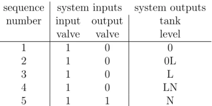
For example, a trace for the process system in Fig. 2.2 filling up a tank with an input and an output valve using the refined qualitative set in Eq.
sequence system inputs system outputs number input output tank
valve valve level
1 1 0 0
2 1 0 0L
3 1 0 L
4 1 0 LN
5 1 1 N
Table 2.1: ”Simple tank fill” operational procedure as a trace (sequence of events). Each row represents a single event with time, input and output states (in a tabular format). System input ”0” means ”closed”, ”1” means
”opened” valve states, while system output ”0” means ”no level”, ”L” means
”low”, ”N” means ”normal” levels in the tank, according to Eq. (2.1)
VA
TA VB
TA LEVEL
Figure 2.2: Single tank process system.
(2.2) can be defined like the one in Table 2.1. In the table each row corre- sponds to a single event in the trace, with its time, inputs and outputs.
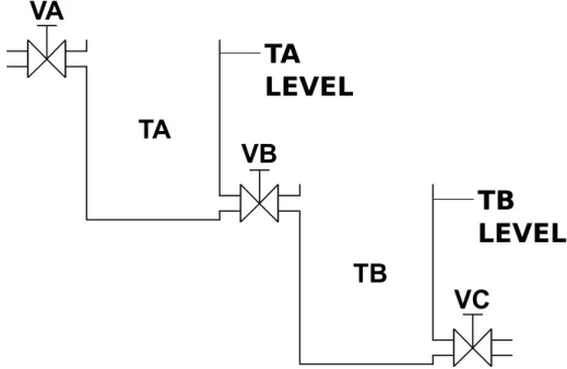
An other trace on Table 2.2, which flushes the liquid from a two/tank sequential process system of Fig. 3.1 can be defined over qualitative set Eq.
(2.1).
Later in the work, a trace describing normal behavior will be called as nominal trace, a trace describing some kind of malfunction or fault will be calledcharacteristic trace, while a trace where it is unknown whether is there a malfunction or not will be called observable ormeasured trace.
sequence system inputs system outputs number VA VB VC TA level TB level
1 0 1 1 N N
2 0 1 1 N N
3 0 1 1 L N
4 0 1 1 0 L
5 0 0 1 0 0
Table 2.2: ”Tank flush” operational procedure as a trace (sequence of events).
Each row represents a single event with time, input and output states (in a tabular format). System input ”0” means ”closed”, ”1” means ”opened”
valve states, while system output ”0” means ”no level”, ”L” means ”low”,
”N” means ”normal” levels in the tank, according to Eq. (2.1)
VA
VB
VC TB
TA
TA LEVEL
TB LEVEL
Figure 2.3: Simple sequential process system with two connected tanks.
2.6 Faults
Faults can be considered as non-observable internal system states of the process system. The general objective of the diagnostics in this work is to determine the values of these hidden internal states. The following simple assumptions are made about the nature and presence of faults:
• All inputs are considered error-free, only outputs of a system may con- tain abnormal values that might refer to a faulty state.
• All fault states permanent in the system during the execution (and the diagnostics) of the operational procedures, random and temporal failures are not considered.
• The structure of the system is assumed to be fixed. We are not dealing with failures which alter the structure as a result.
• Training traces are long enough to capture the transition which will be diagnosed.
• Time is always monotonically increasing and each time instance is present.
• The clock on which all event times are based on is fixed, eg. there is no time skew between any two events of the system.
From the known faults of a process system a diagnoser-specific fault model can be constructed, which can be used during the diagnostics operation in order to detect fault symptoms in measured traces coming from the process system.
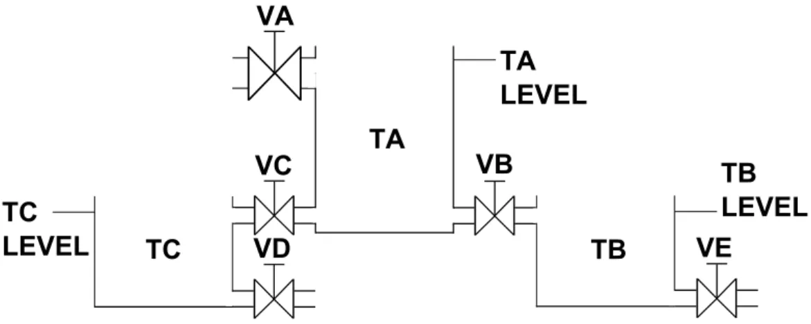
2.7 A simple composite process system
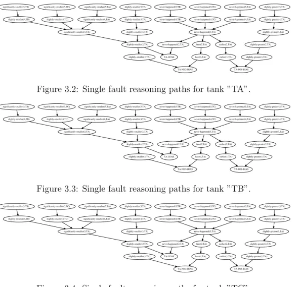
A common example process system is used through the case studies to demon- strate the diagnostic approaches in further chapters. The structure of the process system can be seen in Fig. 3.4. It consists of a main tank ”TA” and two identical auxiliary tanks ”TB” and ”TC” (half the size of the main tank each) connected with pipes to the main tank. All of the pipes have valves on them which can be either open or in closed state. The fluid flows first to the main tank through input valve ”VA”, then leaves it through ”VB” and
”VC” towards the auxiliary tanks. From the auxiliary tanks it flows out of the system via output valves ”VD” and ”VE”.
These basic assumptions are made regarding the operation of this example process system:
1. All valves in the system are assumed to be ”binary”, ie. there are no intermittent states during valve operation.
2. All tanks are equipped with level sensors operating on qualitative range set of Eq. (2.1) or Eq. (2.2).
VA
VC VB VD
TC TB
TA
TA LEVEL
TB LEVEL TC
LEVEL VE
Figure 2.4: Simple process system used for the case studies.
3. Throughout the process system pipe sizes are proportional to the size of the tank they flow into. Due to this, the level in the tanks will be increased by one qualitative level per time instant, provided the input valve is opened and the output valve is closed. If the output and input valves are both in opened state, then the fluid level stays constant in the tank. If only the output valve is opened, then the fluid level will decrease by one qualitative level in the tank per time instant.
2.7.1 Nominal trace
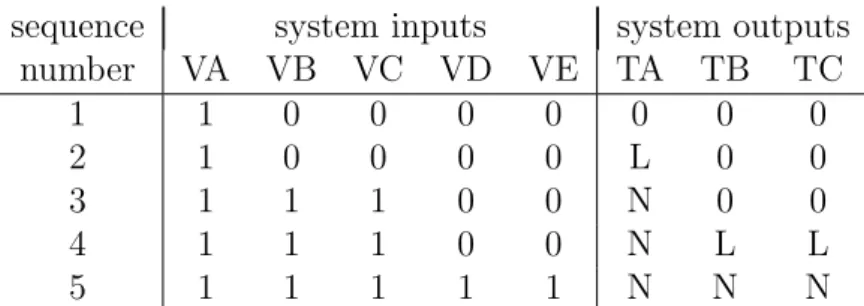
An operational procedure which fills up all three tanks with fluid is used as a common nominal trace to compare the different diagnostic approaches.
Initially all three tanks are empty and all valves are in closed state. After opening input valve ”VA” tank ”TA” is filled up completely with fluid, then valves ”VB” and ”VC” are opened and tanks ”TB” and ”TC” are filled up completely as well. Finally the output valves, ”VD” and ”VE” are opened.
The operational procedure formally can be seen in Table 2.3.
2.7.2 Faults
These types of faults were taken into account for each tank in the example process system:
• The leak of the tank. The size of the leak prevents any fluid from staying inside of the tank, therefore fluid level constantly stays at qual- itative value ”0”.
sequence system inputs system outputs
number VA VB VC VD VE TA TB TC
1 1 0 0 0 0 0 0 0
2 1 0 0 0 0 L 0 0
3 1 1 1 0 0 N 0 0
4 1 1 1 0 0 N L L
5 1 1 1 1 1 N N N
Table 2.3: Nominal trace for the case study. System input ”0” means
”closed”, ”1” means ”opened” valve states, while system output ”0” means
”no level”, ”L” means ”low”, ”N” means ”normal” levels in the tank, ac- cording to Eq. (2.1)
• The positive bias failure of the tank level sensor. The level sensor always detects a qualitative value one degree higher than the actual level of the tank. For instance, given the qualitative set defined in Eq.
(2.1), the level sensor outputs ”N” instead of ”L”.
• The negative bias failure of the tank level sensor. The level sensor always detects a qualitative value one degree lower than the actual level of the tank. For instance, given the qualitative set defined in Eq.
(2.1), the level sensor outputs ”0” instead of ”L”.
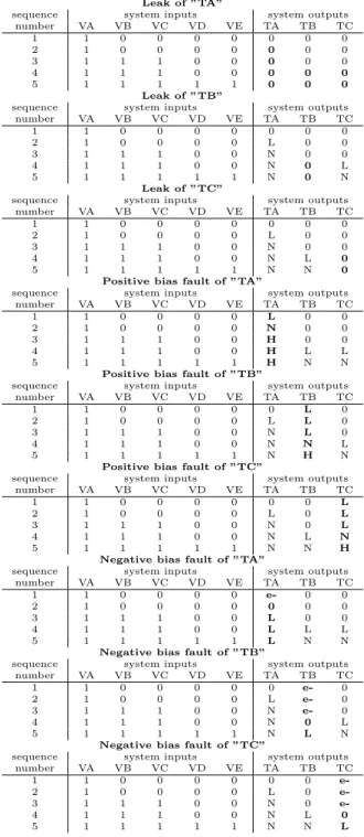
For reference, all faulty traces for the above mentioned single faults are described in Table 2.4.
Dual faults
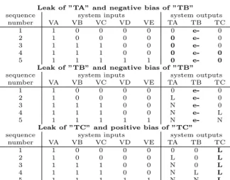
During the presence of dual faults (which are all possible combinations of the above mentioned single faults) the combined effect of the faults on the corresponding output signals will be taken into account. The following apply during the forming of the faulty traces:
• When the faults refer to different output signals (for example, ”TA”
and ”TB”) then the effects of the faulty events are simply combined with each other, this can be done easily due to the fact that they refer to different outputs. For instance, see outputs ”TA” and ”TB” in fault Leak of ”TA” and negative bias of ”TB” in Table 2.5.
• When multiple faults, such as a leak and a positive or negative bias refer to the same output signal (in this case, both to the same tank component) then the effect of faults are combined using the following principles:
Leak of ”TA”
sequence system inputs system outputs
number VA VB VC VD VE TA TB TC
1 1 0 0 0 0 0 0 0
2 1 0 0 0 0 0 0 0
3 1 1 1 0 0 0 0 0
4 1 1 1 0 0 0 0 0
5 1 1 1 1 1 0 0 0
Leak of ”TB”
sequence system inputs system outputs
number VA VB VC VD VE TA TB TC
1 1 0 0 0 0 0 0 0
2 1 0 0 0 0 L 0 0
3 1 1 1 0 0 N 0 0
4 1 1 1 0 0 N 0 L
5 1 1 1 1 1 N 0 N
Leak of ”TC”
sequence system inputs system outputs
number VA VB VC VD VE TA TB TC
1 1 0 0 0 0 0 0 0
2 1 0 0 0 0 L 0 0
3 1 1 1 0 0 N 0 0
4 1 1 1 0 0 N L 0
5 1 1 1 1 1 N N 0
Positive bias fault of ”TA”
sequence system inputs system outputs
number VA VB VC VD VE TA TB TC
1 1 0 0 0 0 L 0 0
2 1 0 0 0 0 N 0 0
3 1 1 1 0 0 H 0 0
4 1 1 1 0 0 H L L
5 1 1 1 1 1 H N N
Positive bias fault of ”TB”
sequence system inputs system outputs
number VA VB VC VD VE TA TB TC
1 1 0 0 0 0 0 L 0
2 1 0 0 0 0 L L 0
3 1 1 1 0 0 N L 0
4 1 1 1 0 0 N N L
5 1 1 1 1 1 N H N
Positive bias fault of ”TC”
sequence system inputs system outputs
number VA VB VC VD VE TA TB TC
1 1 0 0 0 0 0 0 L
2 1 0 0 0 0 L 0 L
3 1 1 1 0 0 N 0 L
4 1 1 1 0 0 N L N
5 1 1 1 1 1 N N H
Negative bias fault of ”TA”
sequence system inputs system outputs
number VA VB VC VD VE TA TB TC
1 1 0 0 0 0 e- 0 0
2 1 0 0 0 0 0 0 0
3 1 1 1 0 0 L 0 0
4 1 1 1 0 0 L L L
5 1 1 1 1 1 L N N
Negative bias fault of ”TB”
sequence system inputs system outputs
number VA VB VC VD VE TA TB TC
1 1 0 0 0 0 0 e- 0
2 1 0 0 0 0 L e- 0
3 1 1 1 0 0 N e- 0
4 1 1 1 0 0 N 0 L
5 1 1 1 1 1 N L N
Negative bias fault of ”TC”
sequence system inputs system outputs
number VA VB VC VD VE TA TB TC
1 1 0 0 0 0 0 0 e-
2 1 0 0 0 0 L 0 e-
3 1 1 1 0 0 N 0 e-
4 1 1 1 0 0 N L 0
5 1 1 1 1 1 N N L
Table 2.4: All single faults as traces in the example case study system. Out- put differences compared to nominal behavior are show inbold.
Leak of ”TA” and negative bias of ”TB”
sequence system inputs system outputs
number VA VB VC VD VE TA TB TC
1 1 0 0 0 0 0 e- 0
2 1 0 0 0 0 0 e- 0
3 1 1 1 0 0 0 e- 0
4 1 1 1 0 0 0 e- 0
5 1 1 1 1 1 0 e- 0
Leak of ”TB” and negative bias of ”TB”
sequence system inputs system outputs
number VA VB VC VD VE TA TB TC
1 1 0 0 0 0 0 e- 0
2 1 0 0 0 0 L e- 0
3 1 1 1 0 0 N e- 0
4 1 1 1 0 0 N e- L
5 1 1 1 1 1 N e- N
Leak of ”TC” and positive bias of ”TC”
sequence system inputs system outputs
number VA VB VC VD VE TA TB TC
1 1 0 0 0 0 0 0 L
2 1 0 0 0 0 L 0 L
3 1 1 1 0 0 N 0 L
4 1 1 1 0 0 N L L
5 1 1 1 1 1 N N L
Table 2.5: A few examples for dual faults in the form of traces. Output differences compared to nominal behavior are shown in bold.
– If the bias is positive then the level sensor constantly shows a qualitative value one degree higher than the empty value. For instance, see output ”TB” in fault Leak of ”TB” and negative bias of ”TB” in Table 2.5 for an example.
– If the bias is negative then the level sensor constantly shows a qualitative value one degree lower than the empty value. For instance, see output ”TC” in faultLeak of ”TC” and positive bias of ”TC” in Table 2.5 for an example.
– It is assumed that the same level sensor cannot have 2 different bias faults (positive and negative) at the same time.
2.8 Summary
In this chapter the basic notions specific to the further described diagnostic approaches were presented. These notions will be used in the coming chapters as a basis, and will be extended with additional method-specific notions there. At the end of the chapter, a simple common case study was presented, which will be used in further chapters to demonstrate the capabilities of the diagnostic methods and to present the main differences between them.
Chapter 3
P-HAZID diagnostics
In this chapter, the procedure HAZID (P-HAZID) methodology, a novel off- line way of reasoning about process system faults during operational proce- dure execution is described in detail. The diagnostics is based upon atomic deviations of measured operational procedure events from the events in a nor- mal procedure. These deviations are organized into a special P-HAZID table which is used by the diagnostic algorithm. When a possibly faulty observable trace need to be diagnosed, its deviations are collected first and using the P-HAZID table, the algorithm can reason about possible fault modes which might have been present in the process system during the execution of the trace.
The chapter is organized into three main parts. First, the notions spe- cific to this methodology, such as the concept of flattening, deviations and the structure of the P-HAZID table is described. Then, the P-HAZID rea- soning algorithm is discussed in detail. Finally, the execution of the method is demonstrated on a simple case study from Section 2.7 and the main char- acteristics of the method are described.
3.1 Introduction
The domain for the usual HAZID analysis is static in the sense, that de- viations from the normal, usually steady-state operation are recorded and used. It is, however, possible to extend the BL-HAZID diagnostic idea (see Section 1.2.1 as well as [42]) to the dynamic case, when the execution of an operational procedure drives the process system from one state to another, and use it for diagnostic purposes. This extended method can be used for finding component faults based on the deviation(s) between the observable inputs and outputs of planned (nominal) and actual (characteristic) event
sequences driven by an operational procedure.
In order to achieve this, a novel dynamic procedure HAZID (P-HAZID) model (in the form of a table) and reasoning method based on the model is proposed in [52]. The use of these P-HAZID tables for diagnostic purposes had been formalized in [44], and it had been extended by taking the structural similarities of process system components into account in [45]. This approach is described in detail in this chapter.
The tabular representation form of the BL-HAZID method (with the columns ”Subsystem”, ”Cause”, ”Deviation” and ”Implication”) is very sim- ilar to the structure of the P-HAZID table (having columns ”Cause”, ”De- viation” and ”Implication”). The difference here is while in the case of BL- HAZID, failures and failure causing events are present in the cells of the table, in the case of the P-HAZID deviations from the nominal operational proce- dure and their root causes are placed in the spreadsheet. The reasoning paths in the P-HAZID method, used for capturing the diagnostics is also analogous to the cause-implication graph of the BL-HAZID, but it describes causal re- lationships between operational procedure deviations and failure root causes.
Similarly, in the case of the BL-HAZID, this graph contains failures, while in the case of the P-HAZID it contains deviations. The P-HAZID methodology can be also thought as an extension of the BL-HAZID methodology with the dimension of time.
On the other hand, the reasoning process in the P-HAZID method is analogous to the widely known concept of if-then or condition-action rules (as described in [41]). In that way it is similar to a G2 (see [14]) based fault diagnostic method described in [35] which transforms the heuristics from a HAZOP table into a set of rules as a fault model and uses if-then rule based backward chaining (see [41]) to diagnose faults in the process system.
Similar to this method, the fault reasoning phase in the P-HAZID can be performed by forward chaining (see [41]) using if-then or condition-action rules (see [41]). The details of this will be further elaborated in Section 3.3.3.
3.2 Basic notions
The most important novel concepts and tools are introduced in this section to formally define the P-HAZID table and the diagnostic method based thereon.
The concepts discussed in this section are the P-HAZID specific extensions of the common notions of event and trace, as described in Section 2.4 and Section 2.5.
event system inputs system outputs sequence input first output second output TA TB
number valve valve valve level level
1 1 0 0 0 0
2 1 0 0 L L
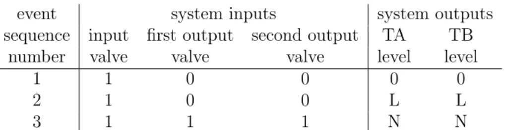
3 1 1 1 N N
Table 3.1: ”Simple tank fill” trace for the process system in Fig. . Each row represents a single event with time, input and output states (in a tabular format). In the system inputs, ”1” means opened, while ”0” means closed state. For the outputs, ”0” means empty, ”L” means low while ”N” means normal level.
3.2.1 Flattening of traces
If there are multiple outputs (as described in Section 2.1) in the process system, then they need to be handled separately in a P-HAZID diagnoser, because the reasoning method works on single output values only. Therefore an initial operation need to be performed for every input trace used by the diagnoser described later. This operation is calledflattening and it works like the following: If there are n outputs in the events of a trace then for every time instant in the tracen number ofsingle-output eventsare generated (note that inputs are considered error-free). These partial events only contain the time instant (sequence number of the whole event), the identifier (index) and the value of the single output. During the generation of deviations, this output value determines the type of the deviation, while the identifier (index) will be the output index of the deviation (as described in Section 3.2.2).
For example, the three-input two-output nominal trace in Table 3.1 will be converted to this sequence of single-output events:
(1;T A: 0),(1;T B : 0),(2;T A:L),(2;T B :L),(3;T A:N),(3;T B :N) After this initial operation the trace will be checked against deviations by comparing it to the flattened form of the nominal trace.
3.2.2 Deviations
Nominal, characteristic and observable traces can be compared by compar- ing their corresponding single-output events acquired after flattening. The difference between two corresponding single-output events (where the time instant is the same) is described by a single deviation. The termdeviation is conceptually analogous to the general term ofservice failure as described in
the common taxonomy (refer to Section 1.3.1 and [7]). Deviations are formed from a deviation guide word (which describes the exact type of the deviation), the time instant to identify the event in the nominal trace and the identi- fier of the output to which the deviation refers to (this is the output of the single-output event). Two major deviation categories can be distinguished, a deviation might be chronological or quantitative. Chronological devi- ations describe that the event regarding that single output in the nominal trace did not occur at the correct time, while quantitative deviations denote the difference in the single output values between events of the same time instant. Both deviation types always refer to a single output variable in the event, if there are more outputs deviating from the nominal event in a measured event then multiple deviations are formed for that event.
The following types of chronological deviations are distinguished (along with their connection with the common taxonomy described in [7]):
• later: When the output value is present in the measured trace, but at alater time instant. According to the common taxonomy this is alate timing fault.
• earlier: When the output value is present in the measured trace, but at anearlier time instant. According to the common taxonomy this is anearly timing fault.
• never-happened: When the particular output value never happened in the measured trace. According to the common taxonomy this is an omission fault, but not necessarily ”human-made”, as it is described there.
The following types of quantitative deviations are used (seeQe in Section 2.1 for an example qualitative set):
• slightly-greater: When an output’s qualitative value is higher than the nominal value and the difference is only one qualitative value.
• significantly-greater: When an output’s qualitative value is higher in the measured event than the nominal one and the difference is more than one qualitative value.
• slightly-smaller: When an output’s qualitative value is lower than the nominal value by one qualitative value.
• significantly-smaller: When an output’s qualitative value is lower in the measured event and the difference is more than one qualitative value.
These deviations are used for capturing small fragments of the fault model (related to specific event pairs of the nominal and measured trace) in a P- HAZID table described in Section 3.2.3.
As an example, the chronological deviation earlier(3;TB) means that the third nominal event, taking only the output value of ”TB” into account, happened at an earlier time instant in the measured trace than in the nominal trace.
As an other example, the quantitative deviationslightly-smaller(4;TA) denotes that at the fourth event in the measured trace the value of output
”TA” was smaller than the value of ”TA” in the same event in the nominal trace and for the same output by one qualitative value.
Note that for a single output value difference in the measured trace a chronological and a quantitative deviation can always be found, denoting the wrong timing of the event (as a chronological deviation) and the incorrect value (as a quantitative deviation) compared to the nominal event. Both of these can be included in the diagnostic reasoning to increase accuracy.
Equality of deviations
During the reasoning procedure the equality of the deviations are checked, in order to match actual deviations with already stored ones. Two deviations are said to be equal if their type, time instant, and output identifier are identical. For example:
• earlier(3;TB) andearlier(3;TB) are equal
• earlier(3;TB) and earlier(3;TC) are not equal because they refer to different outputs (TB and TC)
• earlier(3;TB) and earlier(2;TB) are not equal because they refer to different time instants (3 and 2)
• earlier(3;TB) and later(3;TB) are not equal because they are of dif- ferent type (earlier and later)
Because inputs are considered error-free they are not present in the devia- tions, their values can be determined from the nominal trace and time instant if needed. Only the time instant of the event is used during the reasoning procedure, therefore inputs does not need to be present in the deviations.
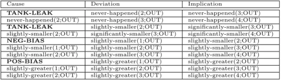
3.2.3 P-HAZID table
As a combination and extension of the widely used FMEA and HAZOP anal- yses (for details, refer to [44] or [12] and partly [42]) the procedure HAZID