MŰHELYTANULMÁNYOK DISCUSSION PAPERS
INSTITUTE OF ECONOMICS, CENTRE FOR ECONOMIC AND REGIONAL STUDIES, HUNGARIAN ACADEMY OF SCIENCES - BUDAPEST, 2018
MT-DP – 2018/17
New and simple algorithms for stable flow problems
ÁGNES CSEH – JANNIK MATUSCHKE
2
Discussion papers MT-DP – 2018/17
Institute of Economics, Centre for Economic and Regional Studies, Hungarian Academy of Sciences
KTI/IE Discussion Papers are circulated to promote discussion and provoque comments.
Any references to discussion papers should clearly state that the paper is preliminary.
Materials published in this series may subject to further publication.
New and simple algorithms for stable flow problems
Authors:
Ágnes Cseh research fellow
Hungarian Academy of Sciences, Centre for Economic and Regional Studies, Institute of Economics
E-mail: cseh.agnes@krtk.mta.hu
Jannik Matuschke postdoc
TUM School of Management and Department of Mathematics, Technische Universität E-mail: jannik.matuschke@tum.de
August 2018
3
New and simple algorithms for stable flow problems Ágnes Cseh – Jannik Matuschke
Abstract
Stable flows generalize the well-known concept of stable matchings to markets in which transactions may involve several agents, forwarding flow from one to another. An instance of the problem consists of a capacitated directed network in which vertices express their preferences over their incident edges. A network flow is stable if there is no group of vertices that all could benefit from rerouting the flow along a walk.
Fleiner [13] established that a stable flow always exists by reducing it to the stable allocation problem.We present an augmenting path algorithm for computing a stable flow, the first algorithm that achieves polynomial running time for this problem without using stable allocations as a black-box subroutine. We further consider the problem of finding a stable flow such that the flow value on every edge is within a given interval. For this problem, we present an elegant graph transformation and based on this, we devise a simple and fast algorithm, which also can be used to find a solution to the stable marriage problem with forced and forbidden edges.
Finally, we study the stable multicommodity flow model introduced by Király and Pap [27].
The original model is highly involved and allows for commoditydependent preference lists at the vertices and commodity-specific edge capacities.
We present several graph-based reductions that show equivalence to a significantly simpler model. We further show that it is NP-complete to decide whether an integral solution exists.
Acknowledgement:
A preliminary version of this paper appeared at the 43rd International workshop on Graph- Theoretic Concepts in Computer Science (WG 2017). The authors were supported by the Hungarian Academy of Sciences under its Momentum Programme (LP2016-3/2016), OTKA grant K128611 and COST Action IC1205 on Computational Social Choice, and by the Alexander von Humboldt Foundation with funds of the German Federal Ministry of Education and Research (BMBF).Keywords : stable flows · restricted edges · multicommodity flows · polynomial algorithm · NP-completeness
JEL: C63, C78
4
Új és egyszerű algoritmusok stabil folyamproblémákra Cseh Ágnes – Jannik Matuschke
Összefoglaló
A stabil folyamprobléma a stabil párosításprobléma egy általánosítása olyan piacokra, amelyeken számos játékos kooperál egymásnak folyamot küldve. A feladat egy inputja egy kapacitással ellátott irányított hálózatból áll, amelyen minden játékos kifejezi a vele szomszédos éleken vett szigorú preferenciáit. Egy hálózati folyam pontosan akkor stabil, ha játékosok egyetlen csoportja sem tud megegyezni egyfajta változtatásban.
Fleiner bebizonyította, hogy stabil folyam mindig létezik a stabil allokációproblémára való visszavezetéssel. Cikkünkben egy augmentáló út típusú algoritmussal számítunk ki egy stabil folyamot, ami az első polinomiális algoritmus a stabil allokációs algoritmus használata nélkül. Ezen felül tanulmányozzuk a tiltott és kötelező élek esetét, azaz amikor a folyamértéknek egy megadott intervallumba kell esnie. A problémát egy elegáns gráftranszformációval oldjuk meg, aminek segítségével egy gyors algoritmust tervezünk.
Végül a Király és Pap által bevezetett többtermékes folyamokat is vizsgáljuk. Az eredeti modell igen bonyolult, amit gráfredukciókkal jelentősen mérsékelünk. Bebizonyítjuk azt is, hogy az egészértékű megoldás találása NP-teljes probléma.
Tárgyszavak: stabil folyam, korlátozott élek, többtermékes folyam, polinomiális algoritmus, NP-teljesség
JEL kódok: C63, C78
Ágnes Cseh · Jannik Matuschke
Abstract Stable flows generalize the well-known concept of stable matchings to markets in which transactions may involve several agents, forwarding flow from one to another. An instance of the problem consists of a capacitated directed network in which vertices express their preferences over their incident edges. A network flow is stable if there is no group of vertices that all could benefit from rerouting the flow along a walk.
Fleiner [13] established that a stable flow always exists by reducing it to the stable allocation problem. We present an augmenting path algorithm for computing a stable flow, the first algorithm that achieves polynomial running time for this problem without using stable allocations as a black-box subroutine. We further consider the problem of finding a stable flow such that the flow value on every edge is within a given interval. For this problem, we present an elegant graph transformation and based on this, we devise a simple and fast algorithm, which also can be used to find a solution to the stable marriage problem with forced and forbidden edges.
Finally, we study the stable multicommodity flow model introduced by Király and Pap [27]. The original model is highly involved and allows for commodity- dependent preference lists at the vertices and commodity-specific edge capacities.
We present several graph-based reductions that show equivalence to a significantly simpler model. We further show that it isNP-complete to decide whether an integral solution exists.
A preliminary version of this paper appeared at the 43rd International Workshop on Graph- Theoretic Concepts in Computer Science (WG 2017). The authors were supported by the Hungarian Academy of Sciences under its Momentum Programme (LP2016-3/2016), OTKA grant K128611 and COST Action IC1205 on Computational Social Choice, and by the Alexan- der von Humboldt Foundation with funds of the German Federal Ministry of Education and Research (BMBF).
Á. Cseh
Hungarian Academy of Sciences, Centre for Economic and Regional Studies, Institute of Eco- nomics, Tóth Kálmán utca 4., 1097 Budapest, Hungary
E-mail: cseh.agnes@krtk.mta.hu J. Matuschke
TUM School of Management and Department of Mathematics, Technische Universität München, Arcisstraße 21, 80333 Munich, Germany
E-mail: jannik.matuschke@tum.de
Keywords stable flows· restricted edges · multicommodity flows· polynomial algorithm·NP-completeness
1 Introduction
Stability is a well-known concept used for matching markets without monetary trans- actions [33]. A stable solution provides certainty that no two agents are willing to selfishly modify the market situation. Stable matchings were first formally defined in the seminal paper of Gale and Shapley [19]. They described an instance of the college admission problem and introduced the terminology based on marriage that since then became wide-spread. Besides this initial application, variants of the sta- ble matching problem are widely used in employer allocation markets [34], university admission decisions [2, 4], campus housing assignments [5, 32] and bandwidth allo- cation [18]. A recent honor proves the currentness and importance of results in the topic: in 2012, Lloyd S. Shapley and Alvin E. Roth were awarded the Sveriges Riks- bank Prize in Economic Sciences in Memory of Alfred Nobel for their outstanding results on market design and matching theory.
In the classic stable marriage problem, we are given a bipartite graph, where the two classes of vertices represent men and women, respectively. Each vertex has a strictly ordered preference list over his or her possible partners. A matching isstable if it is notblocked by any edge, that is, no man-woman pair exists who are mutually inclined to abandon their partners and marry each other [19].
In practice, the stable matching problem is mostly used in one of its capacitated variants, which are the stable many-to-one matching, many-to-many matching and allocation problems. Thestable flow problem can be seen as a high-level generaliza- tion of all these settings. As the most complex graph-theoretical generalization of the stable marriage model, it plays a crucial role in the theoretical understanding of the power and limitations of the stability concept. From a practical point of view, stable flows can be used to model markets in which interactions between agents can involve chains of participants, e.g., supply chain networks involving multiple independent companies.
In the stable flow problem, a directed network with preferences models a market situation. Vertices are vendors dealing with some goods, while edges connecting them represent possible deals. Through his preference list, each vendor specifies how desirable a trade would be to him. Sources and sinks model suppliers and end- consumers. A feasible network flow is stable, if there is no set of vendors who mutually agree to modify the flow in the same manner. A blocking walk represents a set of vendors and a set of possible deals so that all of these vendors would benefit from rerouting some flow along the blocking walk.
Literature review. The notion of stability was extended to so-called “vertical net- works” by Ostrovsky in 2008 [30]. Even though the author proves the existence of a stable solution and presents an extension of the Gale-Shapley algorithm, his model is restricted to unit-capacity acyclic graphs. Stable flows in the more general setting were defined by Fleiner [13], who reduced the stable flow problem to the stable allo- cation problem. Since then, the stable flow problem has been investigated in several papers [15, 16, 24, 29]. Recently, stable flows have been used to derive conflict-free routings in multi-layer graphs [35].
The best currently known computation time for finding a stable flow isO(|E|log|V|) in a network with vertex setV and edge setE. This bound is due to Fleiner’s re- duction to the stable allocation problem and its fastest solution described by Dean and Munshi [8]. Since the reduction takes O(|V|) time, it does not change the in- stance size significantly, and the weighted stable allocation problem can be solved in O(|E|2log|V|) time [8], the same holds for the maximum weight stable flow prob- lem. The Gale-Shapley algorithm can also be extended for stable flows [7], but its straightforward implementation requires pseudo-polynomial running time, just like in the stable allocation problem.
It is sometimes desirable to compute stable solutions using certain forced edges or avoiding a set of forbidden edges. This setting has been an actively researched topic for decades [6, 9, 14, 22, 28]. This problem is known to be solvable in polynomial time in the one-to-one matching case, even in non-bipartite graphs [14]. Though Knuth presented a combinatorial method that finds a stable matching in a bipartite graph with a given set of forced edges or reports that none exists [28], all known methods for finding a stable matching with both forced and forbidden edges exploit a somewhat involved machinery, such as rotations [22], LP techniques [10, 11, 23] or reduction to other advanced problems in stability [9, 14].
In many flow-based applications, various goods are exchanged. Such problems are usually modeled by multicommodity flows [25]. A maximum multicommodity flow can be computed in strongly polynomial time [36], but even when capacities are integer, all optimal solutions might be fractional, and finding a maximum integer multicommodity flow isNP-hard [21]. Király and Pap [27] introduced the concept of stable multicommodity flows, in which edges have preferences over which commodi- ties they like to transport and the preference lists at the vertices may depend on the commodity. They show that a stable solution always exists, but it isPPAD-hard to find one.
Our contribution and structure. In this paper we discuss new and simplified algo- rithms and complexity results for three differently complex variants of the stable flow problem. Section 2 contains preliminaries on stable flows.
• In Section 3 we present a polynomial algorithm for stable flows. To derive an efficient solution method operating directly on the flow network, we combine the well-known pseudo-polynomial Gale-Shapley algorithm and the proposal-refusal pointer machinery known from stable allocations into an augmenting path algo- rithm for computing a stable flow. Besides polynomial running time, the method has the advantage that it is easy to implement and that it provides new insights into the structure of the stable flow problem, which we exploit in later sections.
• Then, in Section 4stable flows with restricted intervalsare discussed. We provide a simple combinatorial algorithm to find a flow with flow value within a pre- given interval for each edge. Surprisingly, our algorithm directly translates into a very simple new algorithm for the problem of stable matchings with forced and forbidden edges in the classical stable marriage case. Unlike the previously known methods, our result relies solely on elementary graph transformations.
• Finally, in Section 5 we studystable multicommodity flows. First, we answer an open question posed in [27] by providing tools to simplify stable multicommodity flow instances to a great extent. In particular, we show that it is without loss of generality to assume that no commodity-specific preferences at the vertices and
no commodity-specific capacities on the edges exist. Then, we reduce 3-satto the integral stable multicommodity flow problem and show that it isNP-complete to decide whether an integral solution exists even if the network in the input has integral capacities only.
2 Preliminaries
Anetwork (D, c) consists of a directed graph D = (V, E) and a capacity function c:E→R≥0 on its edges. The vertex set ofDhas two distinct elements, also called terminal vertices: a source s, which has outgoing edges only and a sink t, which has incoming edges only. Besides differentiating between the source and the sink, we will assume that D does not contain loops or parallel edges, and every vertex v∈V \ {s, t}has both incoming and outgoing edges. These three assumptions are without loss of generality and only for notational convenience. We denote the set of edges leaving a vertexvbyδ+(v) and the set of edges running tovbyδ−(v).
Definition 1 (flow) Function f : E → R≥0 is a flow if it fulfills both of the following requirements:
1. capacity constraints:f(uv)≤c(uv) for everyuv∈E; 2. flow conservation:P
uv∈Ef(uv) =P
vw∈Ef(vw) for allv∈V \ {s, t}.
A stable flow instance is a tripleI= (D, c, r). It comprises a network (D, c) and r, a ranking function that induces for each vertex an ordering of their incident edges.
Each non-terminal vertex ranks its incoming and also its outgoing edges strictly and separately. Formally, r = (rv)v∈V\{s,t}, contains an injective functionrv : δ+(v)∪ δ−(v)→Rfor eachv∈V \ {s, t}. We say thatvprefersedgeetoe0if rv(e)<rv(e).
Terminals do not rank their edges, because their preferences are irrelevant with respect to the following definition.
Definition 2 (blocking walk, stable flow)Ablocking walkof flowfis a directed walkW =hv1, v2, ..., vkisuch that all of the following properties hold:
1. f(vivi+1)< c(vivi+1), for each edgevivi+1,i= 1, ..., k−1;
2. v1=sor there is an edgev1usuch thatf(v1u)>0 and rv1(v1v2)<rv1(v1u);
3. vk=tor there is an edgewvksuch thatf(wvk)>0 and rvk(vk−1vk)<rvk(wvk).
A flow isstable, if there is no blocking walk with respect to it in the graph.
Intuitively, a blocking walk is an unsaturated walk in the graph so that both its starting vertex and its end vertex are inclined to reroute some flow along it.
Notice that the preferences of the internal vertices of the walk do not matter in this definition.
Unsaturated walks fulfilling point 2 are said todominatef at start, while walks fulfilling point 3 dominate f at the end. We can say that a walk blocks f if it dominatesf at both ends.
Problem 1 sf
Input: I = (D, c, r); a directed network (D, c) and r, the preference ordering of vertices.
Question:Is there a stable flowf?
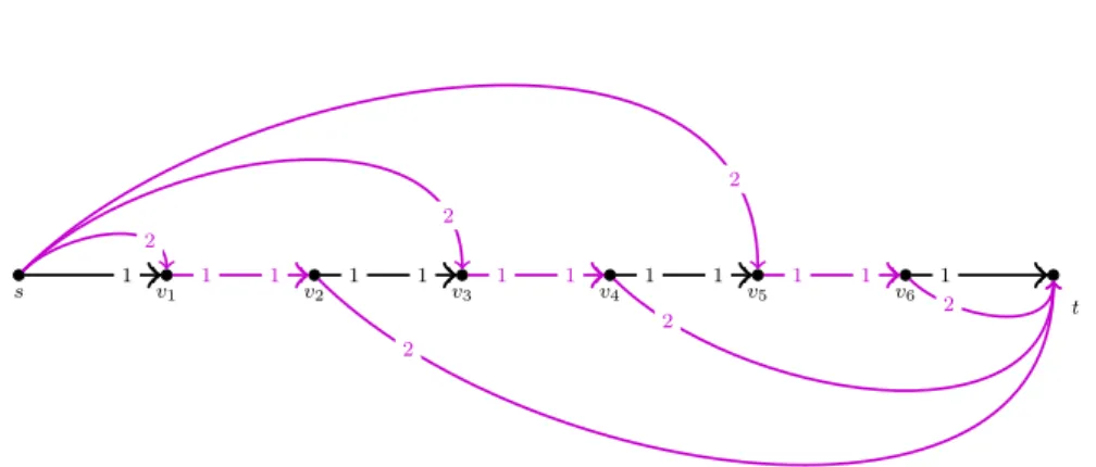
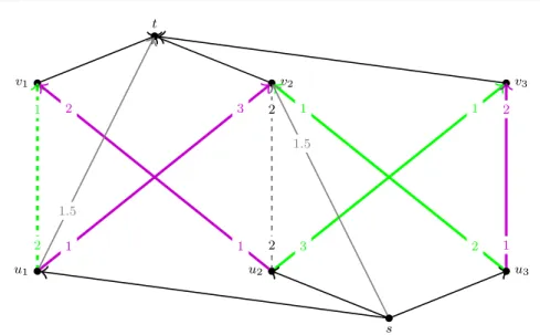
s v1 v2 v3 v4 v5 v6
t
1 1 1 1 1 1 1 1 1 1 1 1
2 2
2
2
2 2
Fig. 1 The maximum flow (marked by colored edges) has value 3 in this unit-capacity network, while the unique stable flow is of value 1 and is sent along the pathhs, v1, v2, ..., ti. It is easy to see that this instance can be extended to demonstrate the ratioΩ(|E|).
Theorem 1 (Fleiner [13])sf always has a stable solution and it can be found in polynomial time. Moreover, for a fixed sfinstance, each edge incident tosorthas the same value in every stable flow.
This result is based on a reduction to the stable allocation problem. The second half of Theorem 1 can be seen as the flow generalization of the so-calledRural Hos- pitals Theorem known for stable matching instances [20]. While Theorem 1 implies that all stable flows have equal value, we remark that this value can be much smaller than that of a maximum flow in the network. In Example 1 we demonstrate a gap ofΩ(|E|).
Example 1 (Small stable flow value)Flows with no unsaturated terminal-terminal paths aremaximalflows. We know that every stable flow is maximal and it is folklore that the ratio of the size of maximal and maximum flows can be of O(|E|). As the instance in Fig. 1 demonstrates, this ratio can also be achieved by the size of a stable flow vs. that of a maximum flow.
3 A polynomial-time augmenting path algorithm for stable flows
Using Fleiner’s construction [13], a stable flow can be found efficiently by computing a stable allocation in a transformed instance instead. Another approach is adapting the widely used Gale-Shapley algorithm tosf. As described in [7], this yields a preflow- push type algorithm, in which vertices forward or reject excessive flow according to their preference lists. While this algorithm has the advantage of operating directly on the network without transformation to stable allocation, its running time is only pseudo-polynomial.
In the following, we describe a polynomial time algorithm to produce a stable flow that operates directly on the network D. Our method is based on the well- known augmenting path algorithm of Ford and Fulkerson [17], also used by Baïou and Balinski [1] and Dean and Munshi [8] for stability problems. The main idea is to introduce proposal and refusal pointers to keep track of possible Gale-Shapley steps and execute them in bulk. Each such iteration corresponds to augmenting flow along ans-t-path or a cycle in a restricted residual network.
3.1 Our algorithm
In the algorithm, every vertex (except for the sink) is associated with two pointers, theproposal pointerand therefusal pointer. Throughout the course of the algorithm, the proposal pointer traverses the outgoing edges of the vertex in order of decreasing preference while the refusal pointer traverses its incoming edges in order of increasing preference. For the sources, we assume an arbitrary preference order. Starting with the 0-flow, the algorithm iteratively augments the flow along a path or cycle in the graph induced by the pointers. This graph consists of the edges pointed at by the proposal pointers and the reversals of the edges pointed at by the refusal pointer.
After each augmentation step, pointers pointing at saturated or refused edges are advanced. The algorithm terminates when the proposal pointer of the source has traversed all its outgoing edges. We prove that when this happens, the algorithm has found a stable flow. As in each iteration, at least one pointer is advanced, the running time of the algorithm is polynomial in the size of the graph. The complete algorithm is listed as Algorithm 1. In the following we describe the individual parts in detail.
Initializing and updating pointers. For notational convenience, we introduce two ar- tificial elements, ∗at the top and ∅at the bottom of each preference list with the convention rv(∗) =−∞and rv(∅) =∞.
Every vertexv∈V \ {t}is associated with aproposal pointer π[v] and arefusal pointer ρ[v], both pointing to elements on the preference list. Initially, π[v] points to the most preferred outgoing edge onv’s preference list, i.e., the entry right after
∗, whereas ρ[v] is inactive, which is denoted by ρ[v] = ∅. We also set ρ[t] = ∅ for notational convenience (we will never changeρ[t] during the algorithm). Note that this implies rv(ρ[t]) =∞.
The pointers atv are advanced through the procedure AdvancePointers(v);
see Algorithm 1, lines 11-17 for a formal listing. A call of this procedure works as follows:
• Ifπ[v] is active, it is advanced to point to the next less-preferred outgoing edge on v’s preference list (lines 12-14). If all ofv’s outgoing edges have been traversed, π[v] reaches its inactive state, i.e., π[v] = ∅, and ρ[v] gets advanced from its inactive state to pointing to the least-preferred incoming edge onv’s preference list. Note that in this latter case, the state ofπ[v] changes from active to inactive between line 12 and line 15, and thus both if-conditions are fulfilled in the same call of the procedure.
• Ifπ[v] is already inactive, the refusal pointerρ[v] gets advanced to the next more- preferred incoming edge on the preference list (lines 15-17). Onceρ[v] traversed
Algorithm 1:Augmenting path algorithm for stable flows
// Initialize proposal pointers to point at most-preferred outgoing edges, refusal pointers inactive.
1 Setπ[v] := argminvw∈Erv(vw) andρ[v] :=∅for allv∈V. 2 Setf:= 0.
// Ensure pointers only point to residual, non-refused edges.
3 while∃uv∈EHπ,ρ withcf(uv) = 0or(π[u] =uvandrv(uv)≥rv(ρ[v]))do 4 AdvancePointers(u)
// Stop once proposal pointer of source becomes inactive.
5 if π[s] =∅then 6 returnf
// Augment flow along path/cycle induced by proposal and refusal pointers.
7 LetW be ans-t-path or cycle inHπ,ρ. 8 Set∆:= mine∈Wcf(e).
9 Augmentf by∆alongW. // Repeat.
10 Goto line 3.
11 procedureAdvancePointers(v)
// If proposal pointer is active, advance it to next less-preferred outgoing edge.
12 ifπ[v]6=∅then
13 SetP :={vw∈E: rv(vw)>rv(π[v])} ∪ {∅}.
14 Setπ[v] := argmine∈Prv(e).
// If proposal pointer has passed all edges, advance refusal pointer to next more-preferred incoming edge.
15 ifπ[v] =∅andρ[v]6=∗then
16 SetR:={uv∈E: rv(uv)<rv(ρ[v])} ∪ {∗}.
17 Setρ[v] := argmaxe∈Rrv(e).
v’s most preferred incoming edge, we setρ[v] =∗, denoting all incoming edges of v have been refused (the procedure will not be called again for this vertex after this point).
The helper graph. With any state of the pointersπ, ρ, we associate a helper graph Hπ,ρ. It has the same vertex set asDand the following edge set:
EHπ,ρ:={π[v] : v∈V \ {t}, π[v]6=∅}
∪ {rev(ρ[v]) : v∈V \ {t}, π[v] =∅, ρ[v]6=∗},
where rev(uv) :=vu denotes the reversal of a given edge. Hence, for every vertex v∈V \ {t}, the graphHπ,ρ either contains the edgeπ[v], if the proposal pointer is still active, or it contains the reversal rev(ρ[v]) of the edgeρ[v], if the refusal pointer is active, or neither of these, if both pointers are inactive. Each edgee∈EHπ,ρ has aresidual capacity cf(e) depending on the current flowf, defined by
cf(e) :=
(
c(e)−f(e) ife∈E,
f(e) ife= rev(e0) for somee0∈E.
s
v
w
t 1
1 1
2 2
1
Fig. 2 Example instance for illustrating a run of Algorithm 1. Numbers next to the vertices indicate preferences of incident edges. Edge capacities arec(sv) = c(vw) = 2 and c(sw) = c(vt) =c(wt) = 1. For the algorithm, we choose the arbitrary preference order of the sources to prefer edgesvoversw.
s
v
w
t 1
1 1
2 2
1
s
v
w
t 1
1 2
1 2
1
s
v
w
t 1
1 2
1 2
1
Fig. 3 The proposal and refusal pointers at the beginning of augmentations 1, 2, and 3, respectively. Proposal pointers are marked by solid black edges, while refusal pointers are the solid gray edges. The dashed edges do not belong to the current set of pointers.
At the beginning of each iteration of the algorithm, we ensure that no proposal or refusal pointer points to an edge with residual capacity 0 and that no proposal pointer points to an edge that has already been refused by its head (lines 3-4).
Augmenting the flow. The algorithm iteratively augments the flowf along ans-t- path or cycleW inHπ,ρ by the bottleneck capacity mine∈Wcf(e) (lines 7-9). Aug- menting a flow f along a path or cycle W by∆ means that for everye∈ W, we increasef(e) by∆ife∈E and decreasef(e0) by ∆ife= rev(e0) for somee0 ∈E. Note that after the augmentation, cf(e) = 0 for at least one edge e∈W, implying that at least one pointer is advanced before the next augmentation. Lemma 2 below shows that an augmenting path or cycle inHπ,ρ exists as long asπ[s] is still active.
The algorithm stops whenπ[s] =∅(lines 5-6).
3.2 Example run of the algorithm
Before we analyze the algorithm, we illustrate it by running it on the example in- stance given in Fig. 2. To each augmentation, the set of pointers is drawn in Fig 3.
Augmentation 1: Initially, the proposal pointers are set to π[s] = sv, π[v] = vw, π[w] = [wt], while all refusal pointers are inactive (pointing to∅). The graph Hπ,ρ
consists of the edges sv, vw, and wt, which comprise a unique s-t-path W1. The algorithm augments f along W1 by its bottleneck capacity 1, yielding the flow f(sv) =f(vw) =f(wt) = 1 andf(sw) =f(vt) = 0.
Pointer update: Because the residual capacity ofwtis 0,AdvancePointers(w) is called. The procedure advancesπ[w] to the inactive state ∅and hence immediately activatesρ[w] withρ[w] =vw. Because alsoπ[v] =vw, this pointer is also advanced according to the second criterion of the while loop. It reachesπ[v] =vt.
Augmentation 2: Withπ[s] =sv,ρ[w] =vw, andπ[v] =vt, the graphHπ,ρconsists of the edgessv, rev(vw) =wv, andvt. The uniques-t-pathW2=hs, v, tiis chosen, the bottleneck capacity iscf(sv) =cf(vt) = 1. After augmentingf alongW2by 1 unit, the new flow isf(sv) = 2, f(vw) =f(vt) =f(wt) = 1 andf(sw) = 0.
Pointer update: Becausecf(sv) = 0, the pointer π[s] is advanced to sw. Because cf(vt) = 0, alsoπ[v] is advanced to ∅andρ[v] gets activated withρ[v] =sv.
Augmentation 3: Withπ[s] = sw, ρ[w] =vw, and ρ[v] =sv, the graph Hπ,ρ con- sists of the edgessw,wv, andvs. These edges comprise the cycleW3. The residual capacities are cf(sw) =cf(wv) = 1 andcf(vs) = 2. Augmenting f along W3 by 1 unit yields the flowf(sv) =f(sw) =f(vt) =f(wt) = 1 andf(vw) = 0.
Pointer update: Becausecf(wv) = 0, the pointer ρ[w] is updated to sv, also trig- gering an update ofπ[s] that was pointing at the same edge. After advancingπ[s] it reaches∅and hence the algorithm terminates.
3.3 Analysis
In the proof of correctness we utilize the following notation. We say the proposal pointer π[v] hasreached edgevw if rv(π[v])≥ rv(vw). We say π[v] has passed the edgevw if rv(π[v]) > rv(vw). We use analogous terms for the refusal pointer ρ[v]
with reversed inequality signs, respectively.
We now make a few observations on the behavior of the pointers. We first ob- serve that π[v] moves from most-preferred to least-preferred edge and ρ[v] moves from least-preferred to most-preferred edge, the ranks of the two pointers are non- decreasing or non-increasing, respectively, during the course of the algorithm (note that the lowest rank inP is always higher than the current rank ofπ[v] in line 13 and the highest rank inRis always lower than the current rank ofρ[v] in line 16).
Observation 1 Throughout the algorithm, rv(π[v]) never decreases and rv(ρ[v]) never increases for anyv∈V \ {t}.
Also, for each vertex, at most one of its two pointers is active at any time, as the refusal pointer is only advanced once the proposal pointer reaches the inactive state.
Observation 2 Throughout the algorithm, for eachv ∈V \ {t}either ρ[v] =∅or π[v] =∅.
Finally, we observe that proposal/refusal pointers do not skip any outgoing/incoming edge, respectively. This is due to the construction ofP in line 13 andRin line 16, which contain every edge that has a rank strictly higher/lower, respectively, than the edge currently pointed at by the pointer.
Observation 3 Letuv∈E.
• If ru(π[u]) < ru(uv) before a call of AdvancePointers(u), then ru(π[u]) ≤ ru(uv)after that call.
• If rv(ρ[v]) > rv(uv) before a call of AdvancePointers(v), then rv(ρ[v]) ≥ rv(uv)after that call.
We next establish a set of invariants that are useful for analyzing the algorithm.
Lemma 1 The following invariants hold true for each uv ∈E any time the algo- rithm is in lines 5-10:
1. Ifrv(ρ[v])≤rv(uv)then π[u]6=uv.
2. Ifrv(ρ[v])<rv(uv)then f(uv) = 0.
3. Ifru(π[u])<ru(uv)thenf(uv) = 0.
4. Ifru(π[u])>rv(uv)then f(uv) =c(uv)or rv(ρ[v])≤rv(uv).
Note that due to the monotonicity of the pointers, once the premise of invariant 1, 2, or 4 is fulfilled for an edge, it will stay this way for the rest of the algorithm.
Intuitively, the invariants state that (1) a proposal pointer does not point to a refused edge, (2) once a refusal pointer has passed an edge, the edge carries no flow, (3) an edge can only carry flow after it is reached by its proposal pointer, and (4) after a proposal pointer has passed an edge, the edge is fully saturated until the refusal pointer of its end not has reached it.
Proof (of Lemma 1) Invariant 1: Note that the pointers are only changed in the while loop in lines 3-4. Ifπ[u] =uv, thenuv∈EHπ,ρ. Therefore the while loop does not terminate whileπ[u] =uvand rv(uv)≥rv(ρ[v]).
Invariant 2: Observe the invariant is true after intialization since f(uv) = 0.
Note thatf(uv) can only increase in line 9 whenπ[u] =uv. In that case, Invariant 1 ensures that rv(ρ[v])>rv(uv). So the invariant can only become invalid by advanc- ing the pointerρ[v] pastuv. Consider the first time this happens in the algorithm.
By Observation 3, this can only happen with a call of AdvancePointers(v) when ρ[v] =uv. But thenπ[v] =∅by Observation 2 and therefore the call of Advance- Pointers(v) can only be triggered by the conditioncf(vu) = 0 of the while loop.
But this impliesf(uv) = 0, so the invariant did not become invalid.
Invariant 3: Initially, f(uv) = 0. The flow can only increase whenuv is part of an augmenting path or cycle in line 9. This can only happen while π[u] = uv by construction ofEHπ,ρ. Because ru(π[u]) is non-decreasing, ru(π[u])≥ru(uv) is true at any time after the first increase off(uv).
Invariant 4: This invariant is true initially because ρ[v] =∅. It can only lose its validity by advancingπ[u] or decreasingf(uv). By Observation 3,π[u] can only pass uvwhenAdvancePointers(u) is called in line 4 whileπ[u] =uv. This call can be triggered because rv(ρ[v])≤rv(uv) or becausecf(uv) = 0 (implyingf(uv) =c(uv)).
In either case, the invariant is not violated. The flow on f(uv) can only decrease when rev(uv)∈W ⊆EHπ,ρ. By definition, this can only happen ifρ[v] =uv, which
is already enough to fulfill the invariant. ut
With the following lemma, we show that, at the beginning of each iteration, the algorithm can actually find ans-t-path or cycle.
Lemma 2 Each time the algorithm reaches line 7, the graphHπ,ρ contains ans-t- path or a cycle.
Proof Consider anyv∈V \ {s, t}at any time the algorithm reaches line 7. We show that ifv has an incoming edge inHπ,ρ, then it also has an outgoing edge in Hπ,ρ. Note that by definition ofEHπ,ρ, the only situation in whichvhas no outgoing edge is whenρ[v] =∗.
Letuv ∈EHπ,ρ be an incoming edge of v. This implies that eitheruv∈E and π[u] =uvorvu∈E andρ[u] =vuby definition ofHπ,ρ.
If π[u] =uv, Invariant 1 of Lemma 1 ensures that rv(ρ[v])>rv(uv) and hence ρ[v]6=∗. Thereforevhas an outgoing edge inHπ,ρ.
If vu∈ E andρ[u] =vu, the termination criterion of the while loop (lines 3-4) guaranteesf(vu) =cf(rev(uv))>0. Hence, by flow conservation,vmust also have an incoming edgeu0v∈E withf(u0v)>0. By Invariant 2 of Lemma 1, this implies ρ[v]6=∗.
Thus every non-terminal vertex with an incoming edge also has an outgoing edge.
Now observe thatπ[s]6=∅ensures thatsalso has an outgoing edge inHπ,ρ. Thus, we can start a walk atsand extend it until we visit a vertex as second time, closing a cycle, or until we reachthaving found ans-t-path. This concludes the proof of the
lemma. ut
Theorem 2 Algorithm 1 computes a stable flow in polynomial time.
Proof We first show that the algorithm indeed computes a stable flow. Assume by contradiction there is a walkW =hv1, v2, . . . , vkiblockingf. We use the previously established invariants to prove the following claim.
Claim For everyi∈ {1, . . . , k−1}, the pointerπ[vi] has passedvivi+1, i.e., rvi(π[vi])>
rvi(vivi+1).
Proof. We show the claim by induction oni. First consider the casei= 1. Due to point 2 in Definition 2, eitherv1=sor rv1(v1v2)<rv1(v1w) for somev1w∈E with f(v1w)>0. In the former case,π[s] has passedv1v2 as the termination criterion of the algorithm impliesπ[s] =∅. In the latter case,f(v1w)>0 implies thatπ[v1] has at least reachedv1wby Invariant 3 of Lemma 1 and thus it has passedv1v2.
Now consider any i∈ {2, . . . , k−1}. Note that by induction hypothesisπ[vi−1] has passedvi−1vi. Furthermoref(vi−1vi)< c(vi−1vi) because no edge ofW is satu- rated. Hence, Invariant 4 of Lemma 1 implies thatρ[vi] must have reachedvi−1vi. In particular,ρ[vi]6=∅and henceπ[vi] =∅by Observation 2, implyingπ[vi] has passed all edges. This completes the induction and proves the claim.
Now considervk, the last vertex ofW. Note that, due to the claim above,π[vk−1] has passedvk−1vk. Furthermore,f(vk−1vk)< c(vk−1vk) as the blocking walk W is unsaturated. Hence, by Invariant 4 of Lemma 1,ρ[vk] has reached at leastvk−1vk, i.e., rvk(ρ[vk])≤rvk(vk−1vk).
Observe that this implies rvk(ρ[vk])<∞= rt(ρ[t]) and thereforevk6=t(remem- ber that ρ[t] = ∅ never changes). Now consider anyuvk ∈ E with rvk(vk−1vk) <
rvk(uvk). Then rvk(ρ[vk]) ≤ rvk(vk−1vk)< rvk(uvk) impliesf(uvk) = 0 by Invari- ant 2 of Lemma 1. ThereforeW does not dominate f at the end, i.e., it does not fulfill point 3 of Definition 2. ThusW is not a blocking walk and the returned flow f is stable.
We now turn to the running time. Note that in every iteration of the while loop (lines 3-4), a pointer of a vertex is advanced. Thus the total number of iterations of the while loop throughout the whole algorithm is bounded by 2|E|by monotonicity of the pointers and the fact that each edge appears in at most two preference lists.
Since every vertex has at most one incoming and one outgoing edge inHπ,ρ by by construction, finding edges violating the termination criterion of the loop can be done in timeO(|V|). The same is true for finding an augmenting path or cycle in line 7.
As after each augmentation, the residual capacity of at least one edge drops to 0, at least one pointer is advanced in line 4 between any two augmentations, limiting the number of augmentations by 2|E|. Hence the total running time of the algorithm is bounded byO(|E||V|). We remark that a more sophisticated implementation using the dynamic-tree data structure can reduce this running time toO(|E|log|V|). How- ever, since our primary aim in this article is to provide new and simple approaches, we omit further investigation of this complication. ut
4 Stable flows with restricted intervals
Various stable matching problems have been tackled under the assumption that re- stricted edges are present in the graph [9, 14]. A restricted edge can be forced or forbidden, and the aim is to find a stable matching that contains all forced edges, while it avoids all forbidden edges. Such edges correspond to transactions that are particularly desirable or undesirable from a social welfare perspective, but it is un- desirable or impossible to push the participating agents directly to use or avoid the edges. We thus look for a stable solution in which the edge restrictions are met voluntarily.
A natural way to generalize the notion of a restricted edge to the stable flow setting is to require the flow value on any given edge to be within a certain interval.
To this end, we introduce alower and anupper bound function.
Problem 1 sf restricted
Input:I= (D, c, r,l,u); ansfinstance (D, c, r), a lower bound functionl:E→R≥0 and an upper bound functionu:E→R≥0.
Question:Is there a stable flowf so thatl(uv)≤f(uv)≤u(uv) for alluv∈E? Note that in the above definition, the upper bound u does not affect blocking walks, i.e., a blocking walk can use edgeuv, even iff(uv) =u(uv)< c(uv) holds. In particular, it is not without loss of generality to assumec(uv) =u(uv) for all edges uv, as decreasingc(uv) may enlarge the set of stable flows.
In the following, we describe a polynomial algorithm that finds a stable flow with restricted intervals or proves its nonexistence. We start with an instance modification step in Section 4.1. Then we prove that restricted intervals can be handled by small network modifications that reduce the problem to the unrestricted version of sf. We show this separately for the case where only forced edges occur, which we callsf forced, in Section 4.2 and for the case where only forbidden edges occur, calledsf forbidden, in Section 4.3. It is straightforward to see that these two results can be combined to solve the general version of sf restricted.
We mention that it is also possible to solvesf restrictedby transforming the instance first into a weightedsfinstance, and then into a weighted stable allocation instance, both solvable in O(|E|2log|V|) time [8]. The advantages of our method
u a b v u v x
y
z
a−ε a a+ε
b−ε b b+ε
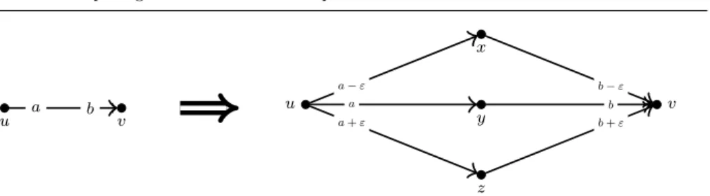
Fig. 4 Splitting an edge with lower and upper bounds. Due to the preferences, capacities and bounds defined on the modified instance, the firstl(uv) units of flow will saturatehu, x, vi, then, the comingu(uv)−l(uv) units of flow will saturatehu, y, vi, and the remainingc(uv)−u(uv) units of flow will usehu, z, vi.
are that it can be applied directly to thesf restricted instance and it also gives us insights to solving the stable roommate problem with restricted edges directly, as pointed out at the end of Sections 4.2 and 4.3. Moreover, our running time is onlyO(|P||E|log|V|), whereP is the set of edges withu(uv)< c(uv).
4.1 Problem simplification
sf restricted generalizes the natural notion of requiring flow to use an edge to its full capacity (by settingl(uv) =c(uv)) and of requiring flow not to use an edge at all (by setting u(uv) = 0), which corresponds to the traditional cases of forced and forbidden edges. In fact, it turns out that any given instance of sf restricted can be transformed into an equivalent instance in whichl(uv),u(uv)∈ {0, c(uv)}for alluv∈E.
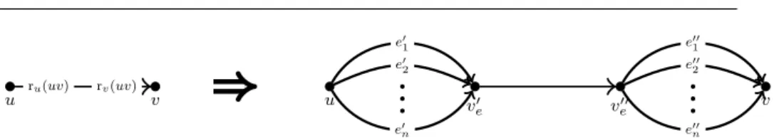
First observe that ifl(uv)>u(uv) for someuv∈E, thensf restrictedtrivially has no solution. Therefore, we henceforth assumel(uv)≤u(uv) for alluv∈E. We further execute the following technical change to the instance in order to obtain an equivalent instance with the desired properties. As shown in Fig. 4, we substitute each edgeuv∈Ewith three parallel paths (to avoid parallel edges):hu, x, vi,hu, y, vi andhu, z, vi. Whileuy andyv take over the rank ofuv,ux andxvare ranked just above,uzandzvare ranked just belowuyandyv. The capacities and bounds of the introduced edges are as follows.
l(ux) = l(xv) = u(ux) = u(xv) = c(ux) = c(xv) = l(uv) l(uy) = l(yv) = 0
u(uy) = u(yv) = c(uy) = c(yv) = u(uv)−l(uv) l(uz) = l(zv) = u(uz) = u(zv) = 0
c(uz) = c(zv) = c(uv)−u(uv)
In words, we split each edgeuv with lower and upper bounds into three paths:
the first pathhu, x, virequires an amount of flow exactly equal to its capacityl(uv), the middle pathhu, y, vihas capacityu(uv)−l(uv) and is unrestricted, the last path hu, z, viwith capacityc(uv)−u(uv) must not carry any flow.
Note that we can map any flow f in original graph to a flow f0 in the modi- fied graph by splitting the flow on each edgeuv into three parts, setting f0(ux) = f0(xv) = min{f(uv),l(uv)},f0(uy) =f0(yv) = min{max{f(uv)−l(uv)),0},u(uv)},
and f0(uz) = f0(zv) = max{f(uv)−u(uv)),0}. Conversely, every flow f0 in the modified instance induces a flow f in the original instance, simply by aggregating the flow values on the three paths, i.e., settingf(uv) =f(ux) +f(uy) +f(uz).
Note that different flows in the modified instance can map to the same flow f in the original network, but it is easy to check that if f is stable, only a unique stable flow in the modified instance maps tof. Thus there is a one-to-one correspon- dence between stable flows in the original instance and in the modified instance.
Furthermore, it is straightforward to check that f respects the bounds l and u in the original instance if and only if f0 does the same in the modified instance. The modified instance is thus equivalent to the original instance.
Remark 1 Note that the encoding size of the modified instance is within a constant factor of the instance size of the original instance. More precisely, the number of edges in the new instance is 6|E|and the number of nodes in the new instance is|V|+ 3|E|, whereV andEare the sets of vertices and edges of the original instance, respectively.
Also the setPof edges withu(e)< c(e) only grows by a factor of 2. Note that because we assumed the original graph to be simple and connected,|V| −1 ≤ |E| ≤ |V|2 and therefore log(|V|+ 3|E|) =O(log|V|). Therefore the asymptotic running time of O(|P||E|log|V|) which we will establish for our algorithm on the modified instance is the same for the original instance.
Henceforth, we will assume that our instances are of this form and use the nota- tion Q:={uv∈E : l(uv) =c(uv)} andP :={uv∈E : u(uv) = 0} for the sets of forced and forbidden edges, respectively.
4.2 Forced edges
In this section we consider an instance ofsf restrictedwhereP =∅. As mentioned earlier, we call this problemsf forced. In Section 4.2.1 we show how to deal with the case|Q|= 1 by reducing the correspondingsf forcedinstance with a single forced edge to an instance of sfwithout forced edges. Then, in Section 4.2.2, we argue that the same technique can be applied to multiple forced edges simultaneously. At last, in Section 4.2.3 we elaborate on the application of our technique for stable matching instances.
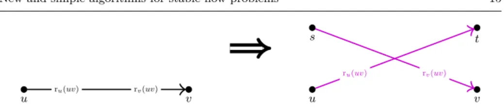
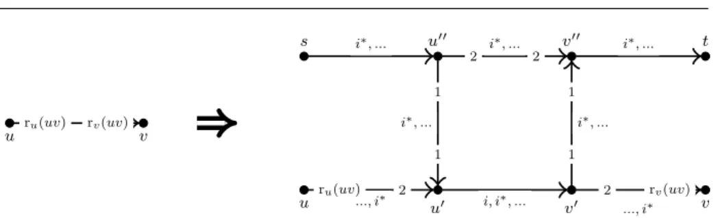
4.2.1 A single forced edge
Let us first consider a single forced edgeuv. We modify graphDto derive a graphD0. The modification consists of deleting the forced edge uv and introducing two new edgessvandutto substitute it. Both new edges have capacityc(uv) and take over uv’s rank onu’s and onv’s preference lists, respectively, as shown in Fig. 5. The rest ofDremains unchanged inD0.
In Lemma 3 we show that flows saturatinguv inDare equivalent to flows satu- rating bothsvandutinD0. Then we refer to the extension of the Rural Hospitals Theorem (Theorem 1) to solve the latter problem.
Lemma 3 Letf be a flow inDwithf(uv) =c(uv). Letf0be the flow inD0 derived by settingf0(sv) =f0(ut) =f(uv)and f0(e) =f(e)for alle∈E\ {uv}. Then f is stable if and only if f0 is stable.
u v
s
u v
t
ru(uv) rv(uv)
rv(uv) ru(uv)
Fig. 5 Substituting forced edgeuvby edgessvandutinD0.
Proof We prove this lemma by showing that walks blockingfalso blockf0and vice versa. We first observe that the set of edges not saturated byf inDis the same as the set of edges not saturated byf0 inD0. This is becauseuvis saturated byf, and thereforeut, sv are saturated byf0, and all other edges are present in both graphs with identical capacities and flow values, respectively. Note that this implies the set of walks in Dnot saturated byf and the set of walks inD0 not saturated byf0 is the same.
Now consider any node u0 ∈ V and any number r > 0. Observe that there is an edgeu0v0 inDwith ru0(u0v0) =r andf(u0v0)>0 if and only if there is u0v00 in D0 with ru0(u0v00) =r andf0(u0v00)>0 (eitheru0v0 itself is in D0 oru0v0 =uv, in which caseu0v00=utfulfills the requirement). Therefore an unsaturated walkW in Ddominatesf at the start if and only if it dominatesf0 at the start. A symmetric argument holds for dominance at the end of an unsaturated walk. This implies that any blocking walk forf inDis a blocking walk forf0inD0 and vice versa. ut Checking the existence of a flow inD0that saturates bothsvandutcan be done by finding any stable flow inD0. This is because Theorem 1 guarantees that all stable flows have the same value on any edge incident tosort.
4.2.2 Multiple forced edges
We observe that we can replace all edges inQone after the other, applying Lemma 3 inductively on the resulting graph. This yields the following theorem.
Theorem 3 LetDQbe the graph obtained fromDwhen replacing each edge inuv∈ Qby edges utand svwith same rank and capacity. LetQ¯ be the set of newly added edges inDQ. Letf be a flow inDsaturating all edges inQ. Then f is stable if and only if the corresponding flowf0 inDQ obtained by settingf0(sv) =f0(ut) =f(uv) for alluv∈Q andf(e) =f0(e)for all e∈E\Q is stable.
In fact, the Rural Hospitals Theorem (Theorem 1) guarantees that either all stable flows in DQ saturate all edges in ¯Q or none does. Thus we can solve sf forcedby a single stable flow computation in DQ.
Theorem 4 sf forcedcan be solved in timeO(|E|log|V|).
Proof AsDQ contains at most twice as many edges asD, we can compute a stable flowf0 inDQin timeO(|E|log|V|), as discussed at the end of Section 3. Iff0(sv) = f0(ut) = c(uv) for all uv ∈ Q, the corresponding flow in D with f(uv) = f0(sv) is a stable flow in D saturating all edges in Q. Now assume f0(sv) < c(uv) or f0(ut)< c(uv) for someuv∈Q. Then by Theorem 1, any stable flow inDQhas this property. Hence, no stable flow inDsaturates all edges inQ. ut
4.2.3 Stable matchings with forced edges
We shortly discuss the case of forced edges in stable matching instances. Notice that our observations are valid in the so-called stable roommates setting, where the underlying graph is not bipartite. The definition of a blocking edge is exactly the same as in the classical bipartite case. An edgeuv /∈ M blocks M if both uandv prefer each other to their respective partners inM.
Problem 2 sr forced
Input:I= (G, r, Q); a graphG(not necessarily bipartite), the preference orderingr of vertices, and a set of forced edgesQ.
Question:Is there a stable matching covering all edges inQ?
The technique described above provides a fairly simple method for solving sr forced, because the Rural Hospitals Theorem holds for the stable roommates prob- lem as well [22, Theorem 4.5.2]. After deleting each forced edge uw ∈ Qfrom the graph, we adduws andutwedges to each of the pairs, where ws andut are newly introduced vertices. These edges take over the rank ofuw. Unlike insf, here we need to introduce two separate dummy vertices to each forced edge, simply due to the matching constraints. There is a stable matching containing all forced edges if and only if an arbitrary stable matching covers all of these new verticesws andut. The proof for this is analogous to that of Lemma 3.
The running time of this algorithm isO(|E|), since it is sufficient to construct a single stable solution in an instance with at most 2|V|vertices. More vertices cannot occur, because in a matching problem more than one forced edge incident to a vertex immediately implies infeasibility. Notice that solvingsr forcedhas the same time complexityO(|E|) as solving the stable roommates problem without any restriction on the edges.
4.3 Forbidden edges
In order to handle sf forbidden, we present here an argumentation of the same structure as in the previous section. In Section 4.3.1, we show how to solve the problem of stable flows with a single forbidden edge by solving two instances on two different extended networks. Then, in Section 4.3.2 we show how these constructions can be used to obtain an algorithm for the case of multiple forbidden edges. Finally, in Section 4.3.3 we discuss the implication of our results to stable matching instances.
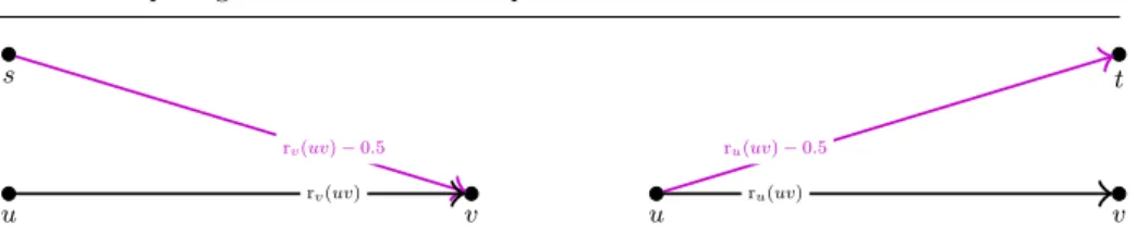
Now we introduce some notation used in this section. We remind the reader that P is the set forbidden edges, where l(e) = c(e). For e= uv ∈ P, we define edges e+ = sv and e− = ut. We set c(e+) = ε > 0 and set rv(e+) = rv(e)−ε, i.e., e+ occurs on v’s preference list exactly before e. Likewise, we set c(e−) = ε and ru(e−) =ru(e)−ε, i.e.,e−occurs onu’s preference list exactly beforee. ForF ⊆P we defineE+(F) :={e+:e∈F}andE−(F) :={e−:e∈F}.
4.3.1 A single forbidden edge
Assume thatP ={e0}for a single edgee0. First we present two modified instances that will come handy when solvingsf forbidden. The first is the graphD+, which