Fixed points and choices:
stable marriages and beyond
Tam´ as Fleiner
A doctoral dissertation
submitted to the Hungarian Academy of Sciences
Budapest, 2018
Contents
Introduction 2
1 Foundations 6
1.1 Stable matchings . . . 6
1.2 Choice functions . . . 7
1.3 Tarski’s fixed point theorem and the deferred acceptance algorithm . . . 10
2 Kernel type results 16 2.1 Poset-kernels . . . 18
2.2 Matroid-kernels . . . 22
3 The structure of kernels 24 3.1 Uncrossing of kernels and median kernels . . . 24
3.2 The splitting property of kernels . . . 25
3.3 Transversals of kernels . . . 27
4 Applications of kernels 29 4.1 Applications on paths. . . 29
4.2 List-edge-colorings . . . 30
4.3 Applications on college admissions. . . 33
5 Stable matching polyhedra 40 5.1 Stable b-matching polyhedra . . . 40
5.2 General kernel-polyhedra . . . 43
6 Stability of network flows 47 7 Nonbipartite stable matchings and kernels 54 7.1 Fractional stable matchings . . . 54
7.2 Reduction of stable matching problems . . . 56
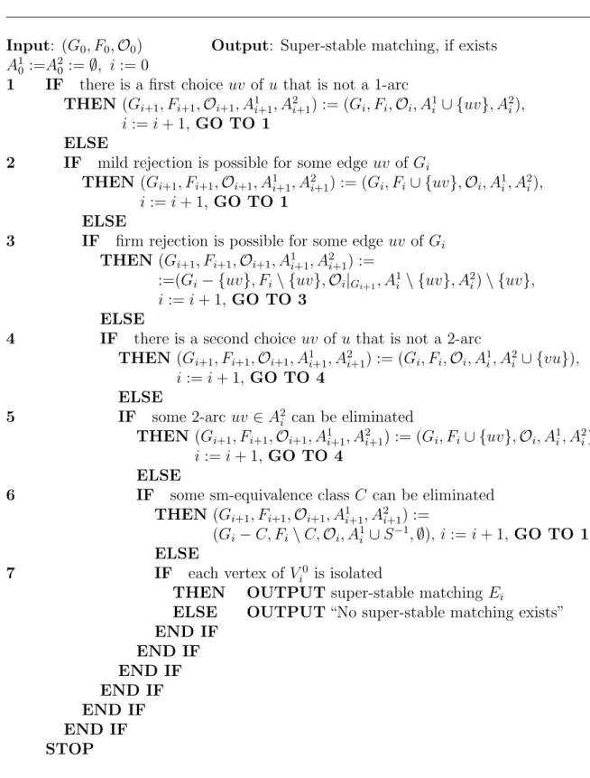
7.3 Extensions of Irving’s algorithm . . . 58
7.3.1 Stable b-matchings . . . 58
7.3.2 Weak preferences and forbidden edges . . . 63
7.4 Roommates with generalized choice functions . . . 70
7.4.1 Complexity issues and structural results . . . 78
Conclusion 85
Introduction
In their famous paper, Gale and Shapley proposed the following problem [35]. Imagine that each of nmen and nwomen ranks the members of the opposite gender as a possible spouse. If these people form n married couples then the hence determined matching is unstable if there is a man and a woman who mutually prefer one another to their eventual partners. A natural goal is to match these people such that this kind of instability does not occur. This idea includes many possible generalizations. The players may seek more than one partners. A practice-motivated example for this is the college admission problem where two the sets of players that rank each other are colleges and applicants instead of men and women, and each college has an individual quota that bounds the number of acceptable applicants from above. In an admission scheme, each applicant is admitted by at most one college and no college exceeds is quota. Such a scheme is unstable if there is an applicant who is not admitted to a certain college but both the college would be happy to accept the applicant (and possibly to fire another less preferred applicant to comply with the quota) and the applicant would improve by being admitted to this college. It is worth mentioning that the admission scheme determined by the education office of the Hungarian government avoids exactly this kind of instability.
It is also possible that not every man-woman (or college-applicant) pair can be real- ized, that is, the bipartite graph representing possible marriages is not a complete one. In fact this graph does not even have to be bipartite. The roommates problem leads to this generalization. In this problem, the goal is to allocate a set of students into two persons dormitory rooms, where each student ranks his or her possible roommates. Instability of a room assignment here means that no two students would be happier to share a room rather that living with their roommates given by the scheme.
A further direction of possible generalizations with a clear practical motivation is dropping the requirement on strict preference orders of the players, and hence allowing ties. For example, in the college admission problem, each applicant is expected to for- mulate a strict preference order on the colleges, while for colleges it is allowed to rank two different applicant equally. As we know, the ranging of each college is based solely on the entrance exam score that might well be equal for two different applicants.
On the original problem the following results are well-known. With the help of the de- ferred acceptance algorithm, Gale and Shapely proved that there exists a stable solution for both the marriage and the college admission problems. Knuth attributes the observa- tion to Conway that stable matchings form a lattice [52]. Later, this observation turned out to be crucial for several further structural results about stable matchings. Actually, the study of stable matchings employs tools of several disciplines: Knuth intended his above mentioned book as an introduction to the theory of algorithms through demon- strating methods and tools in the design and analysis of algorithms [52]. In connection
CONTENTS 3 with further algorithmic complexity aspects, we should mention the book of Gusfield and Irving [37]. Optimization over stable matchings is another natural task, where polyhe- dral methods play an important role here [68, 61, 8, 58, 1, 66, 21]. The book of Roth and Sotomayor leans on notions and methods from Game Theory [60].
Based on our present knowledge, it is fair to say that by the introduction of the notion of stable matchings, Gale and Shapley achieved much more than their direct goal articu- lated in their paper, namely the popularization of the mathematical and game theoretic approach. It becomes clear from the research built upon their work that their notion is exceptionally successful both for practical applications and for theoretical results. For the former fact, we do not need a better argument than the 2012 Nobel Memorial Prize in Economic Sciences having been awarded to Roth and Shapley for their work on mech- anism design and on the theory of stable matchings. A possible example of the latter successes is Galvin’s proof for the Dinitz’ conjecture that essentially leans on stable matchings [36] or the unexpected breakthrough by Kir´aly’s approximation algorithm [49].
It is worth mentioning some results connected to generalizations. The generalized notion of stability may manifest in a common antichain of posets or in a common inde- pendent set of matroids [25], but it is also possible to define stability of network flows that can serve as some model of supply chains known in Economics [23]. Our stable flow model is closely related to the supply chain model by Ostrovsky which is more general in some sense and more restricted in some other sense than flows [55]. As a matter of fact, in the Economics literature, Ostrovsky’s result is considered a clear breakthrough that became the origin of further important results.
These days, stable matchings have a wide literature. Regarding only the algorithmic aspects, the state of the art around 2013 is collected in Manlove’s imposing book [54].
The present work aims for a much more modest goal: it intends to introduce the reader to an unorthodox method and to point out certain interesting aspects. Incidentally, it tries to change our understanding of the history of stable matchings. As we know, Gale and Shapley published their seminal paper in 1962. Later Roth pointed out that a variant of the deferred acceptance algorithm is used in the USA from 1952 [57], hence this should be the origin of the known history of stable matchings. We attempt to date the beginning of the story to as early as 1928 when Knaster and Tarski published (back then without a proof) a fixed point theorem on monotone set functions [51]. Later, in 1955, Tarski proved a lattice theoretical generalization and illustrated its applicability by deducing various mean value theorems known from Analysis [65]. It turned out that this fixed point theorem has nontrivial consequences already in the finite case. It clearly explains the correctness of the deferred acceptance algorithm of Gale and Shapley and the lattice property of stable matchings. As we shall explain, the link between stable matchings and monotone mappings are so-called choice functions introduced by Kelso and Crawford [46].
Without going into the details, we mention some further significant results on general- izations of stable matchings. For some time, it was unclear whether there is a polynomial time algorithm that decides the existence of a stable matching in a nonbipartite graph.
The positive answer is due to Irving whose algorithm has a first phase based on the steps of the deferred acceptance algorithm and in the second phase it eliminates so-called ro- tations until it either finds a stable matching or concludes that no stable matching exists in the input graph [45]. Later, Tan extended Irving’s algorithm and hence he proved the
CONTENTS 4 existence of stable half-matchings (that may contain edges of weight 12 as well) [64]. It also turned out that a graph contains a stable matching if and only if no stable half- matching contains an odd cycle of 12-weight edges. Aharoni and Fleiner have pointed out that the existence of stable half-matchings is a consequence of Scarf’s lemma, and Scarf’s lemma can be regarded as a close relative of Brouwer’s fixed point theorem [6].
Hence, stable matchings can be viewed as fixed points: in case of a bipartite graph, stable matchings are fixed points of a monotone mapping, while in case of nonbipartite graphs, stable matchings are fixed points of a more complicated function. Cechl´arov´a and Fleiner proposed a generalization of Irving’s algorithm to find a stable b-matching [13], while Bir´o, Cechl´arov´a and Fleiner studied the change of stable matchings when a new player emerges on the market. A consequence of their result is that also in case of a nonbipartite graph, it is possible to define a certain friend and an enemy relation between the players by observing how the situation of one player changes when the other player leaves the market [10].
Our present work is structured as follows.
• In Chapter 1, we introduce stable matchings in graphs, build our framework on (lattice-based) choice functions, define choice-function related kernels, and point out that stable matchings are examples of such kernels. Then we introduce Tarski’s fixed point theorem and indicate the connection between fixed points of a mono- tone mapping and the previously defined kernels. In particular, we show that the deferred acceptance algorithm of Gale and Shapley can be regarded as an iteration of a monotone mapping. Our approach described here is an improved version of the one in [20].
• In Chapter2, we deduce two independent results on kernels (i.e. on generalized sta- ble matchings): one about fractional kernels in posets and another one on matroid- kernels.
• Chapter 3is devoted to consequences of the lattice structure of kernels.
• Chapter 4 illustrates three applications: we connect Pym’s linking theorem to kernels, then we prove two extensions of Galvin’s result on list-colorings of graphs and we exhibit an interesting application of the matroid-kernel result on a specific college admission problem with lower quotas.
• Chapter 5 discusses the characterization of kernel-related polyhedra. It turns out that in the general case, a blocking-antiblocking type characterization follows from earlier results of Hoffman and Schwartz on lattice polyhedra and of Fulkerson on blocking polyhedra. In the special case of stable b-matchings, a structural result from Chapter 3 (namely the splitting property) allows us to prove a less implicit characterization based on a polynomial number of constraints.
• Next, Chapter 6is devoted to the recent concept of stability in network flows. We prove that stable flows always exists and exhibit some observations on the structur of stable flows. Our results are closely related to a recent topic in Economics on stability of supply chains that started with the celebrated paper by Ostrovsky [55].
• At last, in Chapter 7, we study stable matchings and generalizations in graphs that are not necessarily bipartite. We point out another fixed-point connection
CONTENTS 5 and show the existence of fractional stable matchings. Then we reduce the problem of stable b-matchings to stable matchings and describe several generalizations of Irving’s algorithm. Our last topic is an extension of Tan’s characterization on stable matchings to the nonbipartite case with choice functions.
• Finally, we conclude with a subjective review on our contribution.
As the goal of the present dissertation is to explain the author’s scientific contribution, we apply the following convention. Results of the author are highlighted by underlining or boxing . Such an expression indicates that the result belongs (at least partly) to the author, in the latter case the result has not been used to obtain a scientific degree so far.
Acknowledgment
The author of this dissertation must thank several people who helped his scientific ca- reer that culminates in the present dissertation. In particular, I am indebted to my high school Maths teacher L´aszl´o Laczk´o, and to L´aszl´o Sur´anyi and Istv´an Reiman for the competition preparation courses. I also learnt a lot from my supervisors Andr´as Frank, Bert Gerards, and Lex Schrijver. Among my collaborators, Katka Cechl´arov´a is clearly the one who influenced my research the most by proposing exciting problems that eventually became publications, by involving me in various research projects, by inviting on working visits infinitely many times, and by helping in all possible ways. Some of the results in this dissertation would not exists without former students P´eter Bir´o and Zsuzsi Jank´o. Though ´Agi Cseh, another former student did not influence the content of this dissertation so much, I really appreciate her help from the background. Perhaps Andr´as Bir´o has the most peculiar contribution towards this dissertation: he pointed out that a generalized version of the Gale-Shapley algorithm that I explained him resembles the fixed point theorem we had at class when proving the Cantor-Bernstein theorem.
Without his insight, my research could have gone on a completely different track. I ac- knowledge all my coauthors, especially Ron Aharoni and David Manlove both of whom I owe a lot. Last but not least I thank the community of the Egerv´ary Research Group for providing an inspiring atmosphere.
Certain organizations also deserve acknowledgement. The Faculty of Electric Engi- neering of the Budapest University of Technology and Economics contributed towards the preparation of the present dissertation by granting a sabbatical leave from February to August 2018. Part of the work described below was supported by the OTKA K108383 and MTA KEP-6/2017 research projects.
Chapter 1 Foundations
In this chapter we introduce our terminology that turns out to be useful in generalizing and extending stable matching related results. First we give a nonstandard proof on the existence of ordinary stable matchings and then we build up our choice function based framework and present the connection to Tarski’s fixed point theorem.
1.1 Stable matchings
Let G = (V, E) be a graph and let v be a linear (preference) order on the set E(v) of edges incident with v for each vertex v of G. We say that edge e is better for v than edge f if e v f holds. Subset M ⊆ E of edges is a matching, if no two edges of M have a common vertex, i.e. if dM(v) ≤ 1 holds or each vertex v ∈ V. For given bounds b : V → N set M ⊆ E of edges is a b-matching if dM(v) ≤ b(v) holds for each vertex v of G. Clearly a matching is a special case of a b-matching for b ≡1. Matching M dominates edge e = uv at u if M contains some edge m with m u f. Similarly, b-matching M b-dominates edge e =uv at u if there are edges m1, . . . , mb(u) of M such that mi u f holds for each 1≤i≤b(u). Matching M (b-)dominates edge e=uv if M (b-)dominatese atu or at v. Edge e blocks (b-)matching M if M does not (b-)dominate e. At last, (b-)matching M is astable (b-)matching if there is no blocking edge, that is, if M dominates each edge of G in E\M. If, for example G is an odd cycle such that each vertex prefers the former vertex to the latter vertex in some orientation of the cycle then it can be seen easily that no stable matching exists in G. This is not the case for bipartite graphs as the following theorem shows.
Theorem 1.1 (Gale and Shapley [35]). If graph G is bipartite then for any prefer- ences there exists a stable matching.
Note that Gale and Shapley proved Theorem 1.1 only for complete bipartite graph Kn,nand they extended this result by showing that there must exist a stableb-matching if b ≡1 on one side ofG. Gale and Shapley actually showed that their deferred acceptance algorithm finds a stable matching for any input instance. This algorithm can be described in man-woman terminology as follows. In the beginning, each man proposes to his first choice. If men propose to different women then proposals become marriages and this is a stable scheme. Otherwise, there is a woman that received more than one proposal. All these women refuse all but their best proposer. If a refusal took place then each man
CHAPTER 1. FOUNDATIONS 7 proposes again to his first choice that did not refuse the particular man. Sooner or later no refusal takes place. The last proposals become marriages and this is output by the algorithm.
In their paper, Gale and Shapley remark that their result is an excellent counterex- ample for the stereotypical beliefs that any reasonable mathematical deduction must contain difficult calculations or obscure formulas. For example, though the description and the proof of correctness of the deferred acceptance algorithm is free of all these, it clearly is a decent mathematical proof. Without disputing this statement, we point out an unusual proof for the correctness of the deferred acceptance algorithm. This is based on the following easy observation that is valid also for nonbipartite graphs.
Lemma 1.2 (Fleiner). Assume that for each vertex v of not necessarily bipartite graph G, linear preference order v is given on the set of edges E(v) incident to v. Assume that e≺v f holds for edge e =uv that is best according to preference order u. Then the set of stable matchings in Gcoincides with the set of stable matchings inG−f. Proof. Let M be a stable matching of G. If e∈M then f 6∈M asM is a matching and if e6∈M then M dominates e atv and hence f 6∈M holds again. Consequently, M is a stable matching of G−f.
Assume now that M is a stable matching of G−f. If e∈ M then M dominates f, and hence M is stable in G, as well. If e6∈M then M must dominatee at v. Therefore M also dominates f atv, and M is a stable matching ofM again.
According to Lemma 1.2, we may remove certain edges from G“for free” without creating or destroying a single stable matching. If we keep on applying this operation on a bipartite graph, sooner or later we reach a state where no more edges can be removed, and hence both men and women have different people on the top of their preference lists. It is easy to see that both the first choices of the men and the first choices of the women represent a stable matching in the graph resulted after all the edge-deletions.
Hence, due to Lemma 1.2, these will be stable matchings also in the original graph G.
Moreover, it also follows immediately that the stable matching output by the deferred acceptance algorithm isman-optimal, meaning that each man receives a wife that is best for him among those women that are achievable for him in some stable matching of G.
Furthermore, this also implies that this procedure provides the worst husband for each woman out of those men that can be the partner of the particular woman in some stable matching of G.
The above proof with obvious changes justifies the correctness of the appropriate extension of the deferred acceptance algorithm for b-matchings and also shows that the output stable b-matching is optimal in the above sense for the proposing side.
Using standard graph-theoretical tools, it is not difficult to prove the following lattice property of stable matchings. IfM1 and M2 are stable (b-)matchings and each man picks his favorite (b-)matching edges out ofM1∪M2 then the hence chosen edges from a stable (b-)matching. Later on, we shall see far reaching generalizations of this fact.
1.2 Choice functions
A most useful tool to study stable matchings and generalizations is the notion of choice functions that helps us to describe the preferences of the players. Our unusual way to
CHAPTER 1. FOUNDATIONS 8 introduce choice functions is based on so-called determinants. For ground setE, mapping F : 2E →2E
• is a choice function if there exists a mapping D : 2E → 2E such that F(X) = X∩ D(X) holds for each subsetX ofE. (Such mapping D is called adeterminant of F);
• is monotone if F(X)⊆ F(Y) holds for X ⊆Y ⊆E and
• is antitone, if F(X)⊆ F(Y) holds whenever Y ⊆X ⊆E and at last
• is substitutable if F is a choice function that has an antitone determinant1.
Obviously,F is a choice function iffF(X)⊆Xholds for any subsetXofE, moreover the same choice function may have several different determinants. The textbook example of a substitutable choice function is the one of men in the Gale-Shapley model.
Example 1.3. Let G= (V, E) be a finite bipartite graph where sets A of men andB of women are the parts and let v be a linear order on the set E(v) of edges incident to v for each vertex v of G. For each subsetX of E, define set FA(X)as those edgese=mw in X that are m-best for man m in X.
It is easy to see that an antitone determinant of the above mapping FA is DA(X) :=
S
v∈A
T
e∈X∩E(v)DA(v, e) whereDA(v, e) := {e0 ∈E(v) :e0 v e} is the set of those edges that are not v-worse for v than e. Hence DA(X) consists of all edges ofE that are not dominated by another edge ofXat some vertex ofA. Similarly, as in Example1.3above, we may define choice function FBof women and the corresponding antitone determinant DB.
Observation 1.4 (Fleiner). Subset M of E is a stable matching in bipartite graph G= (V, E) iff there exist subsets X and Y of E with M =X∩Y and DA(X) =Y and DB(Y) = X hold.
Proof. Assume that M is a stable matching and define X :=DB(M) and Y :=DA(M).
As matching M is stable and no edge e ∈ X \M is dominated by M at a vertex of B, each of these edges are dominated by M at some vertex of A. Consequently, DA(X) = DA(M) =Y. A similar proof shows that DB(Y) = X.
Assume now that M = X ∩Y, DA(X) = Y and DB(Y) = X holds for subsets X and Y of E. If e ≺v f holds for edge e and f of M for some v ∈A then f 6∈ DA(M)⊇ DA(X) = Y, hence f 6∈ X∩Y =M, a contradiction would follow. The same holds in case of v ∈B, so M is a matching.
If f 6∈ M = X∩Y then f 6∈ X = DB(Y) or f 6∈ Y = DA(X). In the first case, f is dominated by some other edge of Y at some vertex v of B. If e denotes the v-best such edge of Y then e ∈ X = DB(Y) and hence e ∈ Y ∩X ∈ M holds, showing that M dominates f at vertexv of B. A similarly proof shows that, in the second case when f 6∈ Y =DA(X) then f is dominated by M at some vertex v of A. Consequently,M is a stable matching.
1The standard definition of substitutability requires thatX∩F(X+e)⊆F(X) holds for anyX⊆E ande∈E. This means that if we are not interested in a certain choice then this choice does not become more interesting if the choices set grows. Our definition is somewhat stronger, but only for an infinite ground setE.
CHAPTER 1. FOUNDATIONS 9 The following useful lemma shows an important property of substitutable choice functions.
Lemma 1.5. If choice function F : 2E →2E is substitutable and F(X)⊆Y ⊆X then F(X)⊆ F(Y) holds.
Proof. For antitone determinant D of F we get F(Y) = Y ∩ D(Y) ⊇ Y ∩ D(X) ⊇ F(X)∩ D(X) = (X∩ D(X))∩ D(X) =X∩ D(X) = F(X).
We define the following crucial properties. Assume that mapping w : 2E → R+ is strictly monotone (that is, w(∅) = 0 and w(a) < w(b) holds whenever a ≺ b). (For a finite set E, w(X) := |X| is an example of such a function, but any positive weight function on E induces such a function.) Choice function F : 2E →2E
• has the IRC property if F(X) = F(Y) holds for F(X)⊆Y ⊆X,
• F is path-independent if X, Y ⊆E ⇒ F(X∪Y) =F(X∪ F(Y)),
• and F is increasing, if |F(X)| ≤ |F(Y)| holds whenever X ⊆Y.
• and F is w-increasing, if w(F(X))≤w(F(Y)) holds whenever X ⊆Y.
Clearly, the increasing property is a special case of the w-increasing one for function w defined by w(X) =|X|.
Observation 1.6 (Fleiner). Let E be a finite set and assume that F : 2E → 2E is a substitutable choice function. Then F has the IRC property if and only if F is path- independent. Moreover, if F is w-increasing for some strictly monotone mapping w on 2E then F has the IRC property (and hence F is path-independent) as well.
Proof. LetD be an antitone determinant of F. AssumeF has the IRC property and let X, Y ⊆E. Clearly,
F(X∪Y) = (X∪Y)∩ D(X∪Y) = (X∩ D(X∪Y))∪(Y ∩ D(X∪Y)⊆
⊆X∪(Y ∩D(X∪Y))⊆X∪(Y ∩ D(Y)) =X∪ F(Y)⊆X∪Y
yielding F(X ∪Y) ⊆ X ∪ F(Y) ⊆ X ∪Y, hence by the IRC property F(X ∪Y) = F(X∪ F(Y)) follows. This means that F is path-independent.
Assume now thatF is path-independent andF(X)⊆Y ⊆X. Path-independence of F implies F(X) =F(X∪Y) =F(F(X)∪Y) = F(Y), hence F has the IRC property.
Assume at last that F is w-increasing and F(X) ⊆ Y ⊆ X. As F(X) ⊆ F(Y) by Lemma 1.5, the w-increasing property of F implies w(F(X))≥ w(F(Y)) and F(X) = F(Y) follows. Hence F has the IRC property, indeed.
Lemma 1.7 (Fleiner, Jank´o [30]). Let E be a finite set and assume that F : 2E → 2E is a substitutable choice function. Then F is path-independent if and only if there exists an antitone determinant DF of F such that
DF(X) =DF(F(X)) holds for any subset X of E . (1.1)
CHAPTER 1. FOUNDATIONS 10 Proof. Assume thatDF is an antitone determinant with property (1.1). LetF(X)⊆Y ⊆ X. By the antitone property of DF we get DF(X) ⊆ DF(Y) ⊆ DF(F(X)) = DF(X) hence DF(X) = DF(Y) holds. Consequently, F(Y) = Y ∩ DF(Y) = Y ∩ DF(X) ⊆ X∩ DF(X) = F(X) and Lemma1.5 impliesF(X) = F(Y). This means that F has the IRC property, hence F is path-independent by Observation 1.6.
Assume now thatF is path-independent with antitone determinantD. Define DF(X) := \
{D(X0) :F(X0) = F(X)} (1.2) for each subset X of E. As F(X) ⊆ DF(X) ⊆ D(X), mapping DF is also a de- terminant of F. By (1.2), DF(X) = DF(Y) holds whenever F(X) = F(Y). So DF(X) = DF(F(X)) follows from path-independence by F(X) = F(∅ ∪X) = F(∅ ∪ F(X)) = F(F(X)). To finish the proof, we have to show that DF is antitone, so as- sume that X ⊆ Y ⊆ E. If F(X0) = F(X) then path-independence of F implies that F(X0∪Y) = F(F(X0)∪Y) =F(F(X)∪Y) =F(X∪Y) =F(Y), hence
DF(X) := \
{D(X0) :F(X0) = F(X)} ⊇\
{D(X0∪Y) :F(X0) = F(X)} ⊇
\{D(X0∪Y) :F(X0∪Y) =F(Y)} ⊇\
{D(Y0) :F(Y0) = F(Y)}=DF(Y) holds, i.e. DF is indeed an antitone determinant of F with property (1.1).
1.3 Tarski’s fixed point theorem and the deferred acceptance algorithm
Poset (L,) is alattice if there is a greatest lower bound (denoted byx∧y) and a least upper bound (denoted by x∨y) for any elements x, y ∈L. Ha a partial order is clear from the context then we may talk about lattice L. Lattice L is complete, if for any subset X of L there exists a greatest lower bound (denoted by V
X) and a least upper bound (denoted by W
X). In case of a complete lattice, 0 and 1 denotes its least and greatest elements, that is, 0 = V
L and 1 = W
L. Clearly, any finite lattice is complete, but not vice verse: finite subsets of N form a lattice on ordinary set inclusion but this lattice has no greatest element, hence it is not complete.
Remark 1.8. Notions defined in section 1.2 can also be defined in the more general setting of lattices by replacing order relation ⊆ by and lattice operations ∩ and ∪ by ∧ and ∨. In section 1.2, we worked out the framework carefully, and we used only operations ∩ and∪ and avoided set-difference. For this reason, our results and proofs in section 1.2 are valid also for choice functions defined on complete lattices.
Our main tool in this work is Tarski’s fixed point theorem about complete lattices.
Note that although we claim corollaries of Tarski’s theorem on ordinary choice functions, these results (with the exception of the second part of Corollary 1.17) are valid in the more general lattice choice function setting, as well.
Theorem 1.9 (Tarski [65]). If F :L→L is a monotone mapping on complete lattice (L,), then fixed points of F form a nonempty complete lattice for order .
CHAPTER 1. FOUNDATIONS 11 Note that in the special case of (L,) = (2E,⊆) Theorem 1.9was proved by Knaster and Tarksi [51]. It is worth observing that in case of a finite lattice, the least fixed point can be constructed as the greatest element of chain 0 F(0) F(F(0)) . . . . (Similarly, the greatest fixed point is the least element of chain 1 F(1) F(F(1)) . . ..) Tarski illustrated the application of Theorem 1.9 by deducing various mean value theorems. Another well-known application, the proof of the Cantor-Schr¨oder-Bernstein theorem also involves infinite lattices. However, Theorem1.9has interesting implications already on finite lattices.
Theorem 1.9 shows that fixed points of a monotone mapping on a complete lattice L form a nonempty lattice subset of L. Our next goal is to prove a strengthening of this result by showing that if a further condition holds then fixed points of a monotone mapping form a sublattice, that is, the lattice operations restricted to fixed points will be the lattice operations on the set of fixed points.
Recall that w : L → R is a strictly monotone function on lattice (L,), that is, w(0) = 0 andw(a)< w(b) holds whenevera≺b. MappingF :L→Lis aw-contraction if
|w(a)−w(b)| ≥ |w(F(a))−w(F(b))| holds for any comparable elements a, b∈L . Theorem 1.10 (Fleiner [20]). If (L,) is a complete lattice, w : L → R+ is strictly monotone function on L and F :L → L is a monotone w-contraction then fixed points of F form a nonempty sublattice of L.
Proof. As the set of fixed points is nonempty by Theorem 1.9, it suffices to prove that fixed points are closed on lattice operations ∧ and ∨ of L. So assume F(a) = a and F(b) = b are fixed points. From a∧b a a∨b we get that F(a∧b) F(a) = a F(a∨b) by monotonicity ofF. SoF(a∧b)a∧band a∨b F(a∨b) and consequently
0≤ |w(a∨b)−w(a)| − |w(F(a∨b))−w(F(a))|
=w(a∨b)−w(a)−(w(F(a∨b))−w(F(a))) =w(a∨b)−w(F(a∨b))≤0 follows asF is aw-contraction andwis strict monotone. So we have equality throughout, in particular w(F(a ∨b)) = w(a ∨ b). Hence F(a ∨b) = a ∨b follows from strict monotonicity of w and a∨b F(a∨b).
By a similar argument, F(a∧b) =a∧b follows from
0≤ |w(a)−w(a∧b)| − |w(F(a))−w(F(a∧b))|
=w(a)−w(a∧b)−(w(F(a))−w(F(a∧b))) =w(a∧b)−w(F(a∧b))≤0. We return to the original lattice version of Tarski’s theorem.
Corollary 1.11 (Fleiner [20]). If F,G : 2E → 2E are substitutable choice functions then there exist subsets X, Y of E such that Y = DF(X) ´es X = DG(Y) holds where DF and DG are antitone determinants of F and G, respectively. Moreover, pairs (X, Y) with this property form a lattice with partial order where (X1, Y1) (X2, Y2) holds whenever X1 ⊆X2 ´es Y2 ⊆Y1.
Proof. Observe that L = (2E × 2E,) is a complete lattice, mapping H(X, Y) :=
(DG(Y),DF(X)) is monotone on L and element (X, Y) ∈ L is a fixed point of H iff Y =DF(X) ´esX =DG(Y) holds. Fixed points of H form a lattice by Theorem 1.9.
CHAPTER 1. FOUNDATIONS 12 Corollary1.11 motivates the following definition.
Definition 1.12. Let F,G : 2E → 2E be substitutable choice functions. Subset K of ground set E is called an F G-kernel if there exist subsets X and Y of E and antitone determinants DF and DG of F and G such that
K =X∩Y, Y =DF(X) and X =DG(Y) (1.3) holds.
Definition1.12 seems to be the right way to generalize the notion of bipartite stable matchings as the example below shows.
Example 1.13. IfFAandFB denotes the preferences of men and women as in Example 1.3 then subset M of E(G) is a stable matching if and only if M is an FAFB-kernel.
It is easy to check that if DA and DB are determinants of FA and FB, respectively then iteration of DB ◦ DA on E(G) is equivalent with the deferred acceptance algorithm of Gale and Shapley.
According to Example 1.13, stable matchings areFAFB-kernels for particular choice functionsFAandFB. As our framework forF G-kernels requires only fairly general prop- erties of choice functions F and G (like substituability, path-independence or eventually increasingness), we will be able to generalize many results on stable matchings in our framework. We continue the study of general F G-kernels.
Observation 1.14 (Fleiner). If (1.3)holds for substitutable choice functions F andG then F(X) = G(Y) = K holds. If F and G are path-independent as well then F(K) = G(K) = K is also true.
Proof. By definition, we have F(X) = X ∩ DF(X) = X ∩Y = K and G(Y) = Y ∩ DG(Y) = Y ∩X = K. If F is path-independent then K =F(X) = F(F(X)) =F(K) and similar holds for G.
Antitone determinants in Definition1.12are not unique in general. However, for path- independent choice functions, this does not matter according to the following lemma.
Lemma 1.15 (Fleiner [20]). LetF,G : 2E →2E be path-independent and substitutable choice functions, let K be an F G-kernel and let DF and DG be antitone determinants of F andG respectively with property (1.1). Then there exist subsets X, Y of E that satisfy (1.3).
Proof. We show that (1.3) holds for X := DG(K) and Y := DF(K). As K is an F G- kernel, we may assume thatK =X0∩Y0 andY0 =D0F(X0),X0 =D0G(Y0) whereD0F and DG0 are antitone determinants of F and G, respectively. By Observation 1.14, as DF is an antitone determinants of F with property (1.1), we get
K =F(X0) =X0 ∩ DF(X0) = X0∩ DF(F(X0)) = X0∩ DF(K) =X0∩Y . Consequently,
G(Y0∪Y) = (Y0 ∪Y)∩ DG0(Y0∪Y)⊆(Y0∪Y)∩ D0G(Y0) =
= (Y0∪Y)∩X0 = (Y0∩X0)∪(Y ∩X0) =K∪K =K ,
CHAPTER 1. FOUNDATIONS 13 hence G(Y0∪Y)⊆K ⊆Y ⊆Y0∪Y and G(Y0∪Y)⊆K ⊆Y0 ⊆Y0∪Y. So by the IRC property of G we have G(Y) = G(Y0 ∪Y) = G(Y0) = K. Property (1.1) of DG implies DG(Y) = DG(G(Y)) = DG(K) = X and a similar proof shows that DF(X) = Y. To finish the proof, we observe that K =G(Y) =Y ∩ DG(Y) = Y ∩X.
The proof of Lemma1.15shows that in case of path-independent substitutable choice functions, F G-kernels are essentially fixed points of a monotone mapping. This is for- mulated in the following lemma.
Lemma 1.16 (Fleiner). If F,G : 2E → 2E are path-independent and substitutable choice functions and DF and DG are their antitone determinants with property (1.1) then DG defines a bijection between F G-kernels and fixed points of mapping DG◦ DF. Proof. We have seen in the proof of Theorem 1.15 that if K is an F G-kernel then X = DG(K) andY =DF(K) satisfy (1.3). AsF(X) =X∩DF(X) =X∩Y =K, determinant DGis injective onF G-kernels. If (1.3) holds forX, Y andKthenDG(DF(X)) = DG(Y) = X, hence F G-kernels are mapped into different fixed points of DG◦ DF. At last, if X is a fixed point of DG◦ DF then (1.3) holds for for Y =DF(X) and K =X∩Y, meaning that DG is indeed a bijection between F G-kernels and fixed points ofDG◦ DF.
Due to Lemmata1.7and1.15, Corollary1.11can be formulated for path-independent choice functions as follows. Function w : 2E → R+ is modular if w(A) + w(B) = w(A∩B) +w(A∪B) holds for any subsets A, B of E. It is easy to see thatw(A) :=|A|
defines a strictly monotone and modular function on 2E.
Corollary 1.17 (Fleiner [20]). If F,G : 2E → 2E are path-independent and substi- tutable choice functions then F G-kernels form a nonempty lattice for partial order F
defined by K1 F K2 whenever F(K1 ∪K2) = K1. Moreover, partial order G is the opposite of F on F G-kernels.
Furthermore, if the above choice functions F and G are also w-increasing for some strictly monotone modular mapping w : 2E → R+ then for any F G-kernels K1, K2 sets K1 ∧F K2 :=F(K1 ∪K2) and K1∨F K2 :=G(K1∪K2) are also F G-kernels such that
χ(K1) +χ(K2) = χ(K1∨F K2) +χ(K1∧F K2) (1.4) holds for the characteristic functions of these kernels. Moreover, w(K1) = w(K2) holds for any F G-kernels K1 and K2.
Proof. Determinant DG defines a bijection between F G-kernels and fixed points of DG◦ DF by Lemma 1.16. As both DG and DF are antitone, their composition is monotone, hence by Theorem 1.9 of Tarski, fixed points of DG◦ DF form a lattice for set-inclusion.
So for the first part of Corollary 1.17, we only have to show that by this bijection, set inclusion corresponds to the partial order given in Corollary 1.17. For this reason, assume that F G-kernels K1 and K2 correspond to X1 = DG(K1), Y1 = DF(K1) and X2 = DG(K2), Y2 = DF(K2), respectively. As we have seen before, F(X1) = X1 ∩ DF(X1) =X1∩Y1 =K1 and F(X2) =K2.
Assume first that F(K1∪K2) = K1. By antitonicity and property (1.1) of DF, Y2 =DF(K2)⊇ DF(K1∪K2) = DF(F(K1∪K2)) =DF(K1) =Y1
CHAPTER 1. FOUNDATIONS 14 and hence X2 = DF(Y2) ⊆ DF(Y1) = X1 follows by the antitone property of DF. A similar proof shows that G(K1∪K2) =K1 implies Y2 ⊆Y1.
Suppose now that X2 ⊆X1 holds. Property (1.1) of DG implies
Y1 =DF(K1) = DF(F(X1)) =DF(X1)⊆ DF(X2) = DF(F(X2) =DF(K2) =Y2 . Now
F(K1∪K2) = F(F(X1)∪ F(X2)) =F(X1∪ F(X2)) =F(X1∪X2) =F(X1) = K1 and
G(K1∪K2) = G(G(Y1)∪ G(Y2)) =G(Y1∪ G(Y2)) =G(Y1∪Y2) =G(Y2) = K2 hold by path-independence of F and G. This justifies the first part of the corollary.
For the second part of the theorem, assume thatF and G are also w-increasing and define D0F and D0G by
D0F(X) =DF(X)∪(E \X) and DG0(Y) =DG(Y)∪(E\Y).
Clearly D0F and D0G are determinants of F and ofG, respectively, and being the union of two antitone mappings, both of them are antitone. We show that both these mappings are w-contractions. Assume thatX ⊆Y holds and observe that
w(X) +DF0 (X) = w(X∩ DF0 (X)) +w(X∪ D0F(X)) =w(F(X)) +w(E)
≤w(F(Y)) +w(E) =w(Y ∩ DF0 (Y)) +w(Y ∪ D0F(Y)) =w(Y) +DF0 (Y)
holds by the modular and strict monotone properties of w. This shows that w(Y)− w(X)≥ D0F(X)− D0F(Y), that is,DF0 is aw-contraction. A similar proof shows thatD0G is also a w-contraction, hence their composition DG0 ◦ D0F is a monotone w-contraction.
Assume now thatF G-kernelsK1 andK2 are determined by setsK1 =X1∩Y1 (with Y1 =DF0 (X1) andX1 =D0G(Y1)) andK2 =X2∩Y2(withY2 =D0F(X2) andX2 =DG0(Y2)).
As X1 and X2 are fixed points of monotone w-contraction DG0 ◦ DF0 , both X1 ∩X2 and X1 ∪X2 are fixed points by Theorem 1.10. Similarly, as Y1 and Y2 are fixed points of monotone w-contractionDF0 ◦ DG0, bothY1∩Y2 and Y1∪Y2 are fixed points of this latter mapping. Consequently, F(X1∪X2) = G(Y1∩Y2) andF(X1∪X2) = G(Y1∪Y2) coincide with F G-kernelsK1∧FK2 andK1∨FK2, moreoverF(X1∪X2) =F(F(X1)∪ F(X2)) = F(K1∪K2) andG(Y1∪Y2) = G(G(Y1)∪G(Y2)) = G(K1∪K2) holds by path-independence of F and G. To finish the proof of the second part, it is left to show (1.4).
The above proof shows that ifF G-kernelsK1 andK2 are determined by pairs (X1, Y1) and (X2, Y2) then K1∧F K2 and K1 ∨F K2 are determined by pairs (X1∪X2, Y1 ∩Y2) and (X1 ∩X2, Y1 ∪ Y2). Consequently, K1 = X1 ∩ Y1, K2 = X2 ∩Y2, K1 ∨F K2 = (X1∪X2)∩Y1∩Y2 and K1∧F K2 =X1∩X2∩(Y1∪Y2). From this latter observation, it is straightforward to check that each element of E contributes the same to both sides of (1.4).
For the last statement, let K1 and K2 be F G-kernels and assume indirectly that w(K1) > w(K2). From modularity of w, (1.4) and the w-increasing property of F and G we get
2·w(K1)> w(K1) +w(K2) =w(K1∧F K2) +w(K1 ∨F K2) = w(F(K1∪K2)) +w(G(K1∪K2))≥w(F(K1)) +w(G(K1)) = w(K1) +w(K1) = 2·w(K1),
CHAPTER 1. FOUNDATIONS 15 a contradiction, proving w(K1) = w(K2) must hold. This finishes the proof of the theorem.
By Corollary1.17, for path-independent substitutable choice functionsF andGonE, there is anF-optimal and aG-optimal F G-kernelKF andKG such thatF(K∪KF) =KF and G(K∪KG) = KG holds for anyF G-kernelK. These F G-kernelsKF and KG are the F-maximal and F-minimal elements of the lattice of F G-kernels.
Let us illustrate Corollary1.17 with the following application.
Example 1.18 (2007 K¨ursch´ak Competition, problem 3).
Prove that any finite subsetH of gridpoints on the plane has a subsetK with the property that
1. any line parallel with one of the axes (i.e. vertical or horizontal) intersects K in at most 2 points,
2. any point of H\K is on a segment with end points in K and parallel with one of the axes.
Proof. Define choice functions F,G : 2H → 2H such that for any subset L of H, F(L) denotes as the set of extreme elements of Lon the horizontal gridlines and G(L) denotes the set of extreme elements of L on the vertical gridlines. It is fairly straightforward to check that F and G are substitutable and path-independent, moreover K satisfies the required properties if K is anF G-kernel. Hence the claim follows from Corollary1.17.
Theorem 1.1 follows immediately from Observation 1.4 and Corollary 1.11. More is true, however. Due to Observation1.4stable matchings coincide withFAFB-kernels that form fixed points of a monotone mapping. These fixed points form a complete lattice by Theorem 1.9 hence there is a least and a greatest fixed point. This immediately implies the existence of a man-optimal stable matching (in which each man is assigned to his best partner he can receive in a stable matching and at the same time each women is matched to her worst stable partner) and the existence of a woman-optimal stable matching (that can be defined by exchanging the role of men and women). It also turns out that the deferred acceptance algorithm of Gale and Shapley can be regarded as the iteration of the monotone mapping DG◦ DF in the proof of Corollary1.17. (We have seen that this iteration finds the least and the greatest fixed point.) It is also not difficult to prove Blair’s theorem on the lattice property from Corollary 1.17.
Theorem 1.19 (Blair [12]). Let G = (V, E) be a bipartite graph with parts A and B and for each vertexv ∈V letFv : 2E(v) →2E(v) a substitutable choice function having the IRC property. Let FA(X) := S{Fv(X∩E(v) :v ∈A} and FB(X) := S{Fv(X∩E(v) : v ∈ B}. Then FAFB-kernels form a nonempty (complete) lattice for partial order B where X B Y holds whenever FB(X∪Y) = X.
Proof . AsFA and FB are substitutable choice functions with the IRC property on 2E, these choice functions are path-independent as well by Observation 1.6. Theorem 1.19 directly follows from Corollary 1.17.
It is worth mentioning that the celebrated ground breaking work of Hatfield and Milgrom [42] is based on the rediscovery of the connection between Corollary 1.17 and Theorem 1.9 of Tarski.
Chapter 2
Kernel type results
We illustrate the choice-function approach by proving a result of Ba¨ıou and Balinski [9] that generalize the theorem on stable b-matchings. Just like several earlier stable matching related results, the proof of Ba¨ıou and Balinski introduces an appropriate gen- eralization of the Gale-Shapley algorithm. Our approach is that we reduce the problem to Corollary 1.17. The choice function in this case works on a complete lattice that is not a subsetlattice. To claim the theorem, we need to fix some terminology.
The stable allocation problem is defined by finite disjoint sets W and F of workers and firms, a map q : W ∪F → R, a set E of edges between W and F along with a map p:E →R and for each worker or firm v ∈W ∪F a linear order <v on those pairs of E that contain v. We shall refer to pairs of E as “edges” and hopefully it will not cause ambiguity. Quota q(v) denotes the maximum of total assignment that worker or firm v can accept and capacity p(wf) of edge e = wf means the maximum allocation that worker w can be assigned to firm f along e. An allocation is a nonnegative map g :E →R such that g(e)≤p(e) holds for each e∈E and for any v ∈W ∪F we have
g(v) := X
x:vx∈E
g(vx)≤q(v) , (2.1)
that is, the total assignment g(v) of playerv cannot exceed quotaq(v) ofv. If (2.1) holds with equality then we say that player v is g-saturated. An allocation isstable if for any edge wf of E at least one of the following properties hold:
eitherg(wf) =p(wf)
(the particular employment is realized with full capacity) (2.2) or P
wf0≤wwfg(wf0) =q(w), that is worker w isg-saturated and w does not
prefer f to any of his employers (we say that wf is g-dominated at w) (2.3) orP
w0f≤fwfg(w0f) =q(f), that is firm f is g-saturated and f does not
prefer w to any of its employees (we say thatwf is g-dominated at f). (2.4) Note that (2.4) and (2.3) imply that if g is a stable allocation, then for each firmf and each worker w
there is at most one edge e dominated at f with g(e)>0 and (2.5) there is at most one edge e dominated at w with g(e)>0 . (2.6)
CHAPTER 2. KERNEL TYPE RESULTS 17 If g1 and g2 are allocations and w ∈ W is a worker then we say that allocation g1 dominates allocation g2 for worker w (in notation g1 ≤w g2) if one of the following properties is true:
either g1(wf) =g2(wf) for each f ∈F or (2.7) P
f0∈Fg1(wf0) = P
f0∈F g2(wf0) = q(w), and
g1(wf)< g2(wf) and g1(wf0)>0 implies that wf0 <w wf. (2.8) That is, if w can freely choose his allocation from max(g1, g2) then w would choose g1 either because g1 andg2 are identical forw or becausewis saturated in both allocations and g1 represents w’s choice out of max(g1, g2). By exchanging the roles of workers and firms, one can define domination relation ≤f for any firm f, as well.
The stable allocation problem was introduced by Ba¨ıou and Balinski as a certain
“continuous” version of the stable marriage problem in [9]. Below we state and prove a nondiscrete generalization of the Ba¨ıou-Balinski result.
Theorem 2.1 (See Ba¨ıou and Balinski [9]). 1. In any stable allocation problem in- stance described by W, F, E, p and q, there exists a stable allocation g. Moreover, if p and q are integral, then there exists an integral stable allocation g.
2. If g1 and g2 are stable allocations and v ∈W∪F then g1 ≤v g2 or g2 ≤v g1 holds.
3. Stable allocations have a natural lattice structure. Namely, if g1 and g2 are stable allocations then g1 ∨g2 and g1∧g2 are stable allocations, where
(g1∨g2)(wf) =
g1(wf) if g1 ≤w g2
g2(wf) if g2 ≤w g1 (2.9) and
(g1∧g2)(wf) =
g1(wf) if g1 ≤f g2 g2(wf) if g2 ≤f g1
(2.10) In other words, if workers choose from two stable allocations then we get another stable allocation, and this is also true for the firms’ choices. Moreover, it is true that
(g1∨g2)(wf) =
g1(wf) if g1 ≥f g2
g2(wf) if g2 ≥f g1 (2.11) and
(g1∧g2)(wf) =
g1(wf) if g1 ≥w g2
g2(wf) if g2 ≥w g1 (2.12) That is, in stable allocation g1∨g2 where each worker picks his better assignment, each firm receives the worse out of the two. Similarly, in g1∧g2 the choice of the firms means the less preferred situation to the workers.
Sketch of the proof of Theorem 2.1. Define lattice Lp = ({l : E → R+, l ≤ p},≤) and observe that Lp is complete. For l ∈ Lp let F(l) denote the choice of workers: if e1 <v
e2 < . . . is the preference order of the edges of E(w) then F(l)(ei) = min l(ei), q(w)−
i−1
X
j=1
F(l)(ej)
! .
CHAPTER 2. KERNEL TYPE RESULTS 18 That is, workers choose their best possible assignment that does not exceed l. In this choices, workers do not care about the firm quotas. By definition, F(l)≤ l, hence F is a choice function on Lp. It is easy to check that F(l) = min(l,DF(l)) where
DF(l)(ei) = max 0, q(w)−
i−1
X
j=1
l(ej)
!
for the above edge ei. Clearly, DF is antitone, hence F is substitutable, and it is also straightforward to see that F is path-independent as well. We can define choice function G and its determinantDG similarly where the role of workers is played by the firms.
To finish the proof, we observe that stable allocations are exactly F G-kernels and Theorem 2.1 follows from Corollary 1.17. The proof of the integrality property in the first part of the theorem is exactly the same, we only have to replace Lp by complete lattice L0p = ({l :E →N, l ≤p},≤).
2.1 Poset-kernels
The fixed-point based approach in Chapter 1 allows us to generalize or extend several earlier results. A common antichain K of finite posets P1 = (E,≤1) and P2 = (E,≤2) is called a P1P2-kernel if for any e ∈E there is some k ∈K such that e ≤1 k ore ≤2 k holds. The first part of the following generalization of Theorem 1.1 of Gale and Shapley can be easily deduced from the result by Sands, Sauer, and Woodrow [62]. (Moreover, it is also true that the Sands-Sauer-Woodrow theorem is a consequence of the first part of Theorem 2.2.)
Theorem 2.2 (Fleiner [20]). For any finite posets P1 = (E,≤1) and P2 = (E,≤2) there exists a P1P2-kernel. Moreover, P1P2-kernels form a lattice for partial order ≺1 where A≺1 A0 holds for two antichains ofP1 if each element of Ahas an≤1-upper bound in A0.
Theorem2.2follows from Corollary1.4and the observation that mapping each subset X of the poset to the set of maxima ofX defines a path-independent choice function. We omit the formal proof as we show a generalization of Theorem 2.2 later in this chapter.
The following application illustrates the first part of Theorem 2.2.
Example 2.3 (2016 K¨ursch´ak Competition, problem 2).
Prove that any finite subset A of the positive integers has a subsetB with the properties below.
• If b1 andb2 are different elements ofB then neitherb1 andb2, nor b1+ 1and b2+ 1 are multiples of one another, and
• for any element a of set A there exists some element b of B such that a divides b or (b+ 1) divides (a+ 1).
Proof. Define two partial orders P1 = (A,≤1) and P2 = (A,≤2) by a≤1 b holds if b | a and a ≤2 b holds if a+ 1 | b + 1. Then subset B of A satisfies the requirements in Example 2.3 if and only ifB is a P1P2-kernel that does exist by Theorem 2.2.
CHAPTER 2. KERNEL TYPE RESULTS 19 Aharoni, Berger, and Gorelik proved a weighted version of Theorem 2.2. We need a couple of definitions to state it. Let P = (V,≤) be a finite poset, let w : V → N be a demand function and let f :V →N be a weight function. For any v ∈V let
f≤↑(v) = max{f(c1) +f(c2) +. . .:v =c1 < c2 < . . .}
denote the maximum weight of chains starting from v. This weight functionf is (≤, w)- independent if
• for any chain c1 < c2 < . . . < ck we have Pk
i=1f(ci)≤max{w(ci) : 1≤i≤k} and
• f(v)·f≤↑(v)≤f(v)·w(v) for any v ∈V.
(The first condition means that the total weight of no chain exceeds the maximal demand of its elements while due to the second condition the total weight of a chain starting at element v of positive weight does not exceed the demand of v.) It is immediate that (≤,1)-independent weight functions coincide with the characteristic vectors of antichains.
The above weight function f w-dominates element c1 of poset P if there is some chain c1 < c2 < . . . < ck such that w(c1)≤ Pk
i=1f(ci) holds, that is, if there is a chain starting at c1 with a total weight not less than the demand of c1. Now let P1 = (V,≤1) and P2 = (V,≤2) be finite posets on common ground set V and let w1, w2 : V → N be two demand functions. By a (w1, w2)-kernel of these posets, we mean a weight function f : V → N that is both (≤1, w1)-independent and (≤2, w2)-independent and moreover f dominates each element of ground set V, more precisely each element of V is w1- dominated by f in P1 orw2-dominated in P2. It is worth observing that a (1,1)-kernel coincides with the previously defined kernel. Now we can claim the theorem on weighted kernels.
Theorem 2.4 (Aharoni, Berger, Gorelik [5]). Let P1 = (V,≤1) and P2 = (V,≤2) be finite posets and let w : V → N be a demand function. Then these posets have a (w, w)-kernel.
An extension of Corollary1.11 of Theorem 1.9 to lattices (according to Remark 1.8) allows us to generalize Theorem 2.4 as follows.
Theorem 2.5 (Fleiner, Jank´o [30]). Let P1 = (V,≤1) and P2 = (V,≤2) be finite posets, and let w1 : V → N and w2 : V → N two demand functions. Then there exists a (w1, w2)-kernel of these posets. The set of (w1, w2)-kernels form a lattice for the partial order 1 of weight functions where f 1 g holds for weight functions f and g if f≤↑1 ≤g≤↑1.
Note that Theorem 2.2 is a special case of Theorem 2.5 for w1 =w2 = 1. Here, we give a sketch of the proof, the interested reader finds the details in [30].
Proof. Let w= max(w1, w2) and define complete latticeLw := ({f :V →N, f ≤w},≤) and refer to the elements of Lw asweight functions. We shall define two choice functions on Lw.
Let V = {v1, v2, . . . , vn} be a linear extension of ≤1, that is, if vi ≤1 vj then j ≤ i holds. (So v1 is ≤1-maximal element of V and vi+1 is a ≤1-maximal element of V \ {v1, v2, . . . , vi} for i = 1,2, . . ..) For weight function f ∈ Lw, define F(f) for values of