A Collection of Constraint Programming Models for the Three-Dimensional Stable Matching Problem with Cyclic Preferences

(1)

for the Three-Dimensional Stable Matching Problem with Cyclic Preferences

Ágnes Cseh

#

Hasso-Plattner-Institute, Universität Potsdam, Germany

Institute of Economics, Centre for Economic and Regional Studies, Pécs, Hungary

Guillaume Escamocher

#

Insight Centre for Data Analytics, School of Computer Science and Information Technology, University College Cork, Ireland

Begüm Genç

#

Luis Quesada

#

Abstract

We introduce five constraint models for the 3-dimensional stable matching problem with cyclic preferences and study their relative performances under diverse configurations. While several constraint models have been proposed for variants of the two-dimensional stable matching problem, we are the first to present constraint models for a higher number of dimensions. We show for all five models how to capture two different stability notions, namely weak and strong stability. Additionally, we translate some well-known fairness notions (i.e. sex-equal, minimum regret, egalitarian) into 3-dimensional matchings, and present how to capture them in each model.

Our tests cover dozens of problem sizes and four different instance generation methods. We explore two levels of commitment in our models: one where we have an individual variable for each agent (individual commitment), and another one where the determination of a variable involves pairing the three agents at once (group commitment). Our experiments show that the suitability of the commitment depends on the type of stability we are dealing with. Our experiments not only led us to discover dependencies between the type of stability and the instance generation method, but also brought light to the role that learning and restarts can play in solving this kind of problems.

2012 ACM Subject Classification Theory of computation→Constraint and logic programming;

Theory of computation→Design and analysis of algorithms

Keywords and phrases Three-dimensional stable matching with cyclic preferences, 3DSM-cyc, Constraint Programming, fairness

Digital Object Identifier 10.4230/LIPIcs.CP.2021.22

Supplementary Material Dataset:https://doi.org/10.5281/zenodo.5156119

Funding This publication has emanated from research conducted with the financial support of Science Foundation Ireland under Grant numbers 12/RC/2289-P2, 16/SP/3804 and 16/RC/3918, which are co-funded under the European Regional Development Fund.

Ágnes Cseh: The Federal Ministry of Education and Research of Germany in the framework of KI-LAB-ITSE (project number 01IS19066), OTKA grant K128611, János Bolyai Research Fellowship.

Acknowledgements COST Action CA16228 European Network for Game Theory.

licensed under Creative Commons License CC-BY 4.0

(2)

1 Introduction

In the classic stable marriage problem, we are given a bipartite graph, where the two sets of vertices represent men and women, respectively. Each vertex has a strictly ordered preference list over his or her possible partners. A matching isstable if it is notblocked by any edge, that is, no man-woman pair exists who are mutually inclined to abandon their partners and marry each other. Stable matchings were first formally defined in the seminal paper of Gale and Shapley [20], who introduced the terminology based on marriage that since then became wide-spread. The notion was then extended to non-bipartite graphs by Irving [27]. Variants of stable matching problems are widely used in employer allocation markets [44], university admission decisions [3, 7], campus housing assignments [8, 42] and bandwidth allocation [19].

Typically, the aim is to solve the decision problem on whether a stable matching exists, or even to solve an optimisation problem considering different fairness notions among stable matchings, such as egalitarian, minimum-regret, or sex-equal.

A natural generalisation of the problem, as suggested by Knuth in his influential book [31], is to extend the two-sided stable marriage problem to three sets of agents. Two input variants of this extension have been defined in the literature. In the first variant, called the3-gender stable marriage problem (3gsm) problem [2, 38], each agent has a preference list over the n²pairs of agents from the other two sets, assuming that each agent set containsnagents.

Another way of generalising stable matching to three agent sets is the3-dimensional stable matching problem with cyclic preferences (3dsm-cyc) [38], in which agents from the first set only have preferences over agents from the second set, agents from the second set only have preferences over agents from the third set, and agents from the third set only have preferences over agents from the first set. In both problem variants, the aim is to find a matching that does not admit a blocking triple, where a blocking triple can have slightly different definitions depending on whether the preference lists contain ties or whether a strict improvement for all agents is required. We explore these different notions in Section 1.1.

1.1 3-dimensional stable matching

In the3gsmproblem variant, the default stability notion is called weak stability, according to which a blocking triple is defined as a set of three agents, all of whom would strictly improve their current match if they would form a triple in the solution. Deciding whether a stable matching exists in a given instance is NP-complete even if the preference lists are complete [38, 47]. A highly restricted preference structure was later identified that allows for a polynomial-time algorithm for the same decision problem [12]. Research then evolved in the direction of preference lists with ties, which gives rise to four different stability definitions, namely weak, strong, super, and ultra stability, and in the direction of consistent preferences, which is a naturally restricted preference domain [26].

The derived research results appear to be more diverse when it comes to the3dsm-cyc problem variant. Firstly, two stability notions have been investigated: weak and strong. A weakly stable matchingdoes not admit a blocking triple such that all three agents would improve, while according tostrong stability, a triple already blocks if at least one of its agents improves, and the others in the triple remain equally satisfied. Biró and McDermid [5]

showed that deciding whether a weakly stable matching exists is NP-complete if preference lists are allowed to be incomplete, and that the same complexity result holds for strong stability even with complete lists. However, the combination of complete lists and weak stability proved to be extremely challenging to solve.

(3)

For this setting, Boros et al. [6] proved that each 3dsm-cycinstance admits a weakly stable matching forn≤3, wherenis the size of each vertex set in the tripartition. Eriksson et al. [15] later extended this result to n≤4. Additionally, Pashkovich and Poirrier [41]

further proved that not only one, but at least two stable matchings exist for each instance withn= 5. By this time, the conjecture on the guaranteed existence of a weakly stable matching in3dsm-cycwith complete lists became one of the most riveting open questions in the matching under preferences literature [31, 33, 50]. Surprisingly, Lam and Plaxton [32]

recently disproved this conjecture by showing that weakly stable matchings for 3dsm-cyc need not exist for an arbitraryn, moreover, it is NP-complete to determine whether a given 3dsm-cycinstance with complete lists admits a weakly stable matching.

Application-oriented research has focused on the so-called “3-sided matching with cyclic and size preferences” problem, defined by Cui and Jia [11]. They modeled three-sided networking services, such as frameworks connecting users, data sources, and servers. In their setting, users have identical preferences over data sources, data sources have preferences over servers based on the transferred data, and servers have preferences over users. The characterising feature of this variant is that a triple might contain more than one user, as servers aim at maximizing the number of users assigned to them. This feature clearly differ- entiates the problem from the classic3dsm-cycsetting. Building upon this work, Panchal and Sharma [40] provided a distributed algorithm that finds a stable solution. Raveendran et al. [43] tested resource allocation in Network Function Virtualisation. They demonstrated the superior performance of the proposed cyclic stable matching framework in terms of data rates and user satisfaction, compared to a centralised random allocation approach.

1.2 Constraint Programming approaches for finding stable matchings

Gent et al. [22] were the first to propose Constraint Programming (CP) models for the classic stable marriage problem. They showed that it is possible to obtain man-optimal and woman-optimal stable matchings immediately from the solution by enforcing Arc Consistency (AC). Later, Unsworth and Prosser [48, 49] presented a binary constraint for the the same problem and showed that their encoding is better in terms of space and time when compared to Gent et al.’s approach. They also investigated sex-equal stable matchings in their studies.

The next milestone was reached by Manlove et al. [34], who proposed three CP models for the Hospital / Residents problem (HR), which is the many-to-one generalisation of the stable marriage problem. They also explored side constraints for their models such as the case with forbidden pairs, residents who may form groups, or residents who may swap their hospitals. The existing research shows that CP models for the stable marriage problem with incomplete lists and for HR are tractable [22, 34]. O’Malley further explored CP models in his thesis for the stable marriage problem, and presented four constraint models [39]. Later on, Siala and O’Sullivan [45] improved the cloned model of Manlove et al. [34] by using a global constraint that achieves Bound Consistency in linear time.

In 2012 Eirinakis et al. [14] used the poset graph of rotations to enumerate all solutions of HR, and presented an improved version to the direct CP model of Manlove et al. [34].

Subsequently, Siala and O’Sullivan [46] used the rotation poset to model stable matchings as SAT formulation for all three types of problems: one-to-one, one-to-many, and many-to-many.

They presented empirical results for finding sex-equal stable matchings, and showed that their approach outperforms the model presented in their previous paper [45]. Additionally, Drummond et al. [13] used SAT encoding for finding stable matchings that include couples.

To the best of our knowledge, CP or SAT models for 3-dimensional stable matchings have not been studied before.

(4)

2 Preliminaries

In this section we introduce the terminology and notation for the problem variants we will study. First we formalise the3dsm-cycproblem and define the two known stability concepts for it. Then, we define three standard fairness notions that were constructed to distinguish balanced stable solutions on bipartite and non-bipartite stable matching instances.

2.1 3-dimensional stable matching with cyclic preferences

Input and output. Formally, a 3dsm-cyc instance is defined over three disjoint sets of agents of sizen, denoted byA={a1, . . . , an},B ={b1, . . . , bn}, and C={c1, . . . , cn}. A matchingM corresponds to a disjoint set of triples, where each triple, denoted by (ai, bj, ck), contains exactly one agent from each agent set. Each agent is equipped with her own preferences in the input. The cyclic property of the preferences means the following: each agent inAhas a strict and complete preference list over the agents inB, each agent inB has a strict and complete preference list over the agents inC, and finally, each agent inC has a strict and complete preference list over the agents inA. These preferences are captured by therank function, where ranka_i(bj) is the position of agentbj in the preference list ofai, from 1 ifbj isai’s most preferred agent tonifbj isai’s least preferred agent.

Preferences over triples. The preference relation of an agent on possible triples can be derived naturally from the preference list of this agent. Agent ai is indifferent between triples (a_i, b_j, c_k₁) and (a_i, b_j, c_k₂), since she only has preferences over the agents inB and the same agentbj appears in both triples. However, when comparing triples (ai, bj₁, ck₁) and (ai, bj₂, ck₂), wherebj₁ ̸=bj₂,ai prefers the first triple if ranka_i(bj₁)<ranka_i(bj₂), and she prefers the second triple otherwise. The preference relation is defined analogously for agents inB andC as well.

Weak and strong stability. A triplet= (a_i, b_j, c_k) is said to be astrongly blocking triple to matchingM if each ofai, bj, and ck prefert to their respective triples inM. Practically, this means thatai, bj, andck could abandon their triples to form triplet on their own, and each of them would be strictly better off int than inM. If a matchingM does not admit any strongly blocking triple, thenM is called aweakly stable matching. Similarly, a triple t= (a_i, b_j, c_k) is called aweakly blocking triple if at least two agents in the triple prefert to their triple inM, while the third agent does not prefer her triple inM tot. This means that at least two agents in the triple can improve their situation by switching tot, while the third agent does not mind the change. A matching that does not admit any weakly blocking triple is referred asstrongly stable. By definition, strongly stable matchings are also weakly stable, but not the other way round. Observe that it is impossible to construct a triplet that keeps exactly two agents of a triple equally satisfied, while making the third agent happier, since the earlier two agents need to keep their partners to reach this, which then already defines the triple as one already inM.

2.2 Fair stable solutions

In this paper, we translate some standard fairness notions from the classic stable marriage problem to3dsm-cyc. In most stable matching problems, several stable solutions might be present, which gives way to choosing a fair or balanced one among them. We now review the most prevalent fairness notions in such decisions [25, 29, 33, 10].

(5)

Egalitarian stable matchings. Possibly the most natural way to define a good stable matching is captured by the notion ofegalitarian stable matchings. Each agent’s satisfaction can be measured by how high she ranks her partner in the matching. In order to gain a comprehensive measure, we sum up those ranks for all matched agents. A stable matching is called egalitarian, if it minimises this sum among all stable matchings. Finding an egalitarian stable matching in the classic stable marriage problem can be done in polynomial time [28, 24], while it is NP-hard, but 2-approximable if the underlying instance is non-bipartite [17, 18].

An egalitarian stable matching in a 3dsm-cycinstance is defined as the extreme point of the following function.

M is a stable matchingmin





 X

(a_i,b_j,c_k)∈M

rankai(bj) + rankbj(ck) + rankc_k(ai)







(1)

Minimum regret stable matchings. Another popular fairness notion, calledminimum regret stable matching, intuitively maximises the satisfaction of the least satisfied person in the instance. In this context, each agent’s regret is measured by how high she ranks her partner in the matching – the larger this rank is, the more regret she experiences. The regret of matching M is defined as the largest regret in the instance, i.e. the worst rank that appears in the matching. Finding a minimum regret stable matching can be done in polynomial time both in bipartite and non-bipartite instances [23, 24]. A minimum regret stable matching in a 3dsm-cycinstance is defined as the extreme point of the following function.

min

M is a stable matching

max

(ai,bj,ck)∈M

rank_a_i(b_j),rank_b_j(c_k),rank_c_k(a_i)

(2)

Sex-equal stable matchings. A third condition is calledsex-equality, which aims at reaching the same satisfaction level of each agent set. The satisfaction of a set of agents is measured by summing up the satisfaction level, that is, the rank of the matching partner, of each agent in the set. In the classic stable marriage setting, a sex-equal stable matching minimises the difference between the satisfaction level of the two sets. Finding a sex-equal stable matching is NP-hard in those instances [30, 35]. Even though the notion cannot be defined for non-bipartite instances, it translates readily to3dsm-cyc instances. The difference of satisfaction level between any two of the three agent sets can be computed exactly as in the classic stable marriage setting. Then, the sum of the three pairwise differences must be minimised. We define a sex-equal stable matching as the extreme point of the following function.

min

M is a stable matching

(

X

(a_i,b_j,c_k)∈M

rank_a_i(b_j)−rank_b_j(c_k)

+

X

(ai,bj,ck)∈M

rankb_j(ck)−rankc_k(ai)

+

X

(ai,bj,ck)∈M

rankc_k(ai)−ranka_i(bj)

)

(3)

(6)

2.3 Our contribution

This paper is the first to model 3-dimensional stable matchings, specifically the3dsm-cyc problem, including its optimisation variants using side constraints. We propose the following CP models to find a stable matching in the3dsm-cyc problem: div(divided agent sets), uni(unified agent sets), andhs(hitting set). We implement each one of the models under both weak and strong stability. For thediv anduni models, we investigate two kinds of domain values: one based on the unique identifiers of the agents themselves, referred as agent-based (agents), and the other based on the ranks of agents in one’s preference list, referred asrank-based (ranks). We first use the models to find any satisfying solution to a given3dsm-cycinstance. Subsequently, we extend all models to optimisation variants under different fairness criteria and conclude with some empirical findings.

3 Methodology

In this section we present the details of our five proposed models. For each model, we propose the mandatory matching and stability constraints. We also propose how to model the fairness constraints for different optimisation versions. Furthermore, if we identified any, we state the redundant constraints that help the models with better pruning the search space.

3.1 Agent-based DIV model

The div-agents model consists of 3n variables X = {x1, . . . , xn}, Y = {y1, . . . , yn}, and Z = {z₁, . . . , z_n}, where the domain of each variable v is set as D(v) = {1, . . . , n}. For agent-based domain values, assigningxi =j (respectivelyyi=j, orzi=j) corresponds to matchinga_i tob_j (respectivelyb_i toc_j, orc_i toa_j). A stable matchingM, if any exists, is found by using the following constraints.

(matching) For all 1≤i, j, k≤n, we add the constraintxi=j∧yj =k⇒zk =i. This is to ensure that each solution corresponds to a feasible, if not stable, matching.

(stability) Under weak stability, for all 1 ≤ i, j, k ≤ n, and for all i^′, j^′, k^′ such that a_i prefersb_j tob_j^′, b_j prefers c_k to c_k^′ and c_k prefers a_i to a_i^′ we add the constraint xi ̸=j^′∨yj ̸=k^′∨zk ̸=i^′. This is to ensure that there is no strongly blocking triple.

When solving the problem under strong stability, the condition to post the constraint becomes: ai prefersbj to bj^′ or j^′=j, and bj prefersck to ck^′ or k^′=k, andck prefers ai toai^′ or i^′=i, andi^′̸=i∨j^′̸=j∨k^′̸=k. Here, as well as in the other models, the difference between weak and strong stability constraints is that the latter also cover the case when exactly two agents of a potential blocking triple are matched together.

(redundancy) For all 1≤i, j, k≤n, we add the constraint y_j=k∧z_k=i⇒x_i=j.

(redundancy) For all 1≤i, j, k≤n, we add the constraint zk =i∧xi=j⇒yj=k.

(redundancy) We add AllDifferent(X) and AllDifferent(Y) and AllDiffer- ent(Z) to ensure each agent has exactly one partner from each set.

(optimisation) When solving a fair version of the problem, we add a constraint to minimise the objective in one of the following ways, depending on which notion of fairness is desired:

For egalitarianM, we model Eqn. 1 as: P(rank_a_i(b_j) + rank_b_j(c_k) + rankc_k(a_i)) for alli, j, k such thatxi=j∧yj=k∧zk =i.

For minimum regret M, we model Eqn. 2 as: max(max(ranka_i(bj), rankb_j(ck), rankck(ai))) for alli, j, ksuch that xi=j∧yj=k∧zk=i.

(7)

For sex-equal M, we model Eqn. 3 as:

SA−SB

+

SB −SC

+

SC−SA

where SA=P(ranka_i(bj)) for alli, jsuch thatxi =j,SB=P(rankb_j(ck)) for allj, ksuch that y_j =k, andS_C=P(rank_c_k(a_i)) for all k, isuch thatz_k=i.

3.2 Rank-based DIV model

Variables and domains are the same in the rank-baseddivmodel (div-ranks) as they are in the agent-baseddivmodel (div-agents), but this time assigningx_i=j (respectivelyy_i =j, or zi =j) corresponds to matchingai to herj^th preferred agent (respectivelybi to herj^th preferred agent, orc_i to herj^th preferred agent), who might be different fromb_j. A stable matchingM, if any exists, is found by using the following constraints.

(matching) For all 1 ≤ i, j, k ≤ n, we add the constraint x_i = rankai(b_j)∧y_j = rankb_j(ck) ⇒ zk = rankc_k(ai). This is to ensure that each solution corresponds to a feasible, if not stable, matching.

(stability) Under weak stability, for all 1 ≤ i, j, k ≤ n, we add the constraint xi ≤ rank_a_i(b_j)∨y_j≤rank_b_j(c_k)∨z_k≤rank_c_k(a_i). This is to ensure that there is no strongly blocking triple. When solving the problem under strong stability, the inequalities are strict but the following part is added to each disjunction: ∨(x_i = rank_a_i(b_j)∧y_j = rankb_j(ck)∧zk= rankc_k(ai)).

(redundancy) For all 1 ≤ i, j, k ≤ n, we add the constraint y_j = rank_b_j(c_k)∧z_k = rankc_k(ai)⇒xk = ranka_i(bj).

(redundancy) For all 1 ≤ i, j, k ≤ n, we add the constraint z_k = rank_c_k(a_i)∧x_i = ranka_i(bj)⇒yj= rankb_j(ck).

(optimisation) We add a constraint to minimise the objective in one of the following ways, depending on which notion of fairness is desired:

For egalitarianM, we model Eqn. 1 as: Pn

i=1(x_i+y_i+z_i).

For minimum regretM, we model Eqn. 2 as: max(max(xi, yi, zi)) for all 1≤i≤n.

S_A−S_B +

S_B −S_C +

S_C−S_A where SA=Pn

i=1(xi),SB=Pn

j=1(yj), andSC=Pn k=1(zk).

Note that, as opposed to agent-based domains, there are noAllDifferent constraints in rank-based models. The reason for this is that with rank-based domains it is possible for two agents in the same agent set to be assigned the same value, for example if they both got assigned to their most preferred agent.

3.3 Agent-based UNI model

Theuni-agents model consists ofnvariablesX={x1, . . . , xn}, where the domain of each variablev is set asD(v) ={(1,1), . . . ,(1, n),(2,1), . . . ,(n, n)}. Each tuple domain variable is implemented as an integer domain variable by representing the tuple (j, k) with the integer (j−1)n+k. For agent-based domain values, assigning (j, k) toxi corresponds to having the triple (a_i, b_j, c_k) in the matching. A stable matchingM, if any exists, is found by using the following constraints.

In both the current and following subsections, we denote by xi,B and xi,C respectively the first and second elements of the pair assigned tox_i.

(matching) For all 1≤i < i^′ ≤n, we add the constraintxi,B̸=xi^′,B∧xi,C ̸=xi^′,C. This is to ensure that each solution corresponds to a feasible, if not stable, matching.

(8)

(stability) Underweak stability, for all 1≤i, j, k≤n, for all 1≤i^′, i^′′, j^′, k^′ ≤n such thatai prefersbj tobj^′,bj prefersck tock^′ andck prefersai toai^′, we add the constraint (x_i,B ̸=j^′)∨(x_i^′′ ̸= (j, k^′))∨(x_i^′_,C ̸=k). This is to ensure that no triple is blocking.

Because in UNI only the agents fromAhave their own associated variables, determining whether b_j was assigned toc_k^′ requires checking for each agenta_i^′′ fromAwhether both bj andck^′ were assigned to ai^′′. This is the reason for the additional indexi^′′. When solving the problem understrong stability, the condition to post the constraint becomes:

ai prefersbj tobj^′ orj^′=j, andbj prefersck tock^′ ork^′=k, andck prefersaitoai^′ or i^′=i, and i^′̸=i∨j^′̸=j∨k^′̸=k.

(redundancy) We impose the constraintAllDifferent(X).

(redundancy) Denote byF(i) the set of tuples that have an agentias their first element, andS(i) the tuples that have i as their second. Then, for all agents ∀i ∈ n we have P

j∈F(i)Count(j, X) = 1 andP

j∈S(i)Count(j, X) = 1.

For egalitarian M, we model Eqn. 1 as: Pn

i=1(rank_a_i(b_x_i,B) + rank_b_xi,B(c_x_i,C) + rankc_xi,C(ai)).

For minimum regret M, we model Eqn. 2 as: max(max( ranka_i(bx_i,B), rankb_xi,B(cx_i,C),rankc_xi,C(ai))) for all 1≤i≤n.

For sex-equalM, we model Eqn. 3 as:

SA−SB

+

SB−SC

+

SC−SA

whereSA= Pn

i=1(ranka_i(bx_i,B)),SB =Pn

i=1(rankb_xi,B(cx_i,C)), andSC=Pn

i=1(rankc_xi,C(ai)).

3.4 Rank-based UNI model

Variables and domains are implemented the same in the rank-basedunimodel (uni-ranks) as they are in the agent-basedunimodel (uni-agents), but this time assigning (j, k) toxi

corresponds to matchingai to herj^th preferred agent fromB, and matching the latter to herk^th preferred agent fromC. A stable matchingM, if any exists, is found by using the following constraints.

(matching) For all 1≤i < i^′≤n, we add the constraint pref_a_i(xi,B)̸= pref_a

i′(xi^′,B)∧ pref_pref

ai(x_i,B)(x_i,C) ̸= pref_pref

ai′(x_i′,B)(x_i^′_,C), where pref_a

i(r) (respectively pref_b

j(r), or pref_c

k(r)) represents the agent b ∈ B (respectively c ∈ C, or a ∈ A) such that ranka_i(b) =r(respectively rankb_j(c) =r, or rankc_k(a) =r). This is to ensure that each solution corresponds to a feasible, if not stable, matching.

(stability) Under weak stability for all 1 ≤ i, j, k ≤ n, for all 1 ≤ i^′, i^′′, j^′′ ≤ n such thatc_k strictly prefers a_i toa_i′, we add the constraint (x_i,B ≤rankai(b_j))∨(x_i′′,B ̸=

ranka_i′′(bj))∨(xi^′′,C ≤rankb_j(ck))∨(xi^′ ̸= (ranka_i′(bj^′′),rankb_j′′(ck))). This is to ensure that no triple is blocking. When solving the problem understrongstability,c_k’s preference ofai toai^′ is not strict (i^′ can be equal toi) but the two inequalities are, and to each disjunction is added the following part: ∨(x_i= (rank_a_i(b_j),rank_b_j(c_k))).

For egalitarianM, we model Eqn. 1 as: Pn

i=1(xi,B+xi,C+ rankpref_pref

ai(xi,B)(x_i,C)(ai)).

For minimum regret M, we model Eqn. 2 as: max(max(xi,B, xi,C, rank_pref

prefai(xi,B)(x_i,C)(a_i))) for all 1≤i≤n.

S_A−S_B +

S_B−S_C +

S_C−S_A where SA=Pn

i=1(xi,B),SB =Pn

i=1(xi,C), andSC=Pn

i=1(rank_pref_pref

ai(xi,B)(x_i,C)(ai)).

(9)

3.5 HS model

In thehs model, letT be the set of all possible triples as {(1,1,1),(1,1,2), . . . ,(n, n, n)}.

Without loss of generality, assume that the triples in T are ordered, so t_i∈T refers to the i^th triple ofT. Given a triplet∈T, we denote byBT(t) all the triples inT that preventt from becoming a blocking triple given the preferences. Then, finding a stable matching is equivalent to finding a hitting set of the non-blocking triples inT.

LetM be a set variable whose upper bound is {i:ti∈T}.

(matching) Ensure that each agent from each set is matched by having:

∀a∈A:P

ti∈T:a∈ti(i∈M) = 1;

∀b∈B :P

t_i∈T:b∈ti(i∈M) = 1;

∀c∈C:P

t_i∈T:c∈ti(i∈M) = 1.

(stability) The stable matching is a hitting set of the non-blocking triples: ∀tj ∈ T : M ∩ {i:ti∈BT(tj)} ̸=∅. The type of stability is addressed in the computation of the BT sets. The model as such is not concerned with this aspect.

In this model,M is constrained to be a set of triples representing the stable matching as defined in Section 2.2, so egalitarianM, minimum regretM, and sex-equalM are defined as in Equations 1, 2, and 3 respectively.

In the actual implementation, M is represented in terms of an array of n³ Boolean variables, where each variable refers to the inclusion/exclusion of the corresponding tuple in the mapping.

4 Experiments

We performed our experiments on machines with Intel(R) Xeon(R) CPU with 2.40GHz running on Ubuntu 18.04. Our initial experiments on small instances comparing all models are performed using Gecode 6.3.0 [21]. Then, we conduct further experiments by using our best performing models for larger instances on a constraint solver based on lazy-clause generation, namely Chuffed 0.10.4. [9]. Fordivandunimodels, instances were first processed by MiniZinc 2.5.5 [37] before being given to the solvers. Thehs model has been directly encoded using Gecode 6.2.0. In Section 4.1 we describe the datasets in use. Then, in Sections 4.2 and 4.3 we compare the proposed models.

4.1 Dataset description

For every sizen present in our experiments, we generated 100 instances withnagents in each agent set and a complete list for each agent. Half of these instances are random and the other half have some or all of the preferences based on master lists. Master list instances are instances where the preference lists of all agents in the same agent set are identical. Master lists provide a natural way to represent the fact that in practice agent preferences are often not independent. Examples of real-life applications of master lists occur in resident matching programs [4], dormitory room assignments [42], cooperative download applications such as BitTorrent [1], and 3-sided networking services [11]. The detailed distribution of the 100 instances generated for each size is as follows:

Random: 50 random instances from uniform distribution.

ML_oneset: 20 instances where the preference lists of the agents in one of the agent sets are based on master lists, and the preference lists of the agents in the other two agent sets are random.

(10)

ML_1swap: 15 instances, where each agent set has a randomly chosen master list that all agents in the set follow. Then, we randomly choose two agents from each agent’s preference list, and swap their positions.

ML_2swaps: 15 instances, where each agent set has a randomly chosen master list that all agents in the set follow. First, we randomly choose two agents from each agent’s preference list, and swap their positions. Subsequently, we randomly choose two more agents from each list such that the new agents were not involved in the first swap, then we swap their positions.

Note that neither the type of stability (weak or strong) nor the fairness objective is part of the preferences themselves. For this reason, the 100 instances generated for each sizen are used for both types of stability and for all satisfiability and optimisation versions.

We did not consider instances where all preference lists in all three sets are exact master lists, because the complete set of stable matchings for these instances is known [16].

ML_oneset instances always have a strongly stable matching (Lemma 1), but, contrary to the case with master lists in all three sets, not all solutions have been characterised. Therefore there is value in modelling fairness versions of the problem for instances with this structure.

4.2 Model comparison

In this section, we first test each one of our five models (i.e.hs, div-agents, div-ranks, uni-agents, anduni-ranks) using different heuristic search strategies on small instances in Gecode to find out which strategy performs best. In Gecode experiments, we did not use extra propagation techniques such as lazy clause generation or restarts. Considering that thehs model is implemented in Gecode, and not all search strategies are common to both Gecode and MiniZinc, for a fair comparison between all five models we used indomain_min (assigning the smallest value in the domain) and indomain_max (assigning the largest value in the domain) strategies combined with a search on variables in the given order. The former is referred asnonemin, and the latter asnonemax. Additionally, we further tested thediv andunimodels using alternative built-in search strategies that exist in MiniZinc, notably indomain_split, a heuristic that bisects a variable’s domain then tries the lower half before trying the upper one. We observed that a strategy that is based on choosing the variable with the smallest domain size using indomain_min results in the best performance fordiv model, while using indomain_split instead of indomain_min leads to the best performance forunimodel. We refer to these asfailmin andfailsplit strategies, respectively. Therefore, all the remaining results and plots were obtained by running hs with nonemax strategy, div-agents anddiv-ranks with failmin, anduni-agents anduni-ranks with failsplit.

During the experiments, we used a time-limit of 10 minutes for each instance. Considering the huge number of all combinations of different parameters in each model, we adapted a look-ahead approach for our tests, i.e. we started performing tests on all models using small instancesn= 4. Then, we incremented thenfor each model that has the potential to be the best. If a model times out on most of the instances for a given combination of parameters, we do not test it further on these instances.

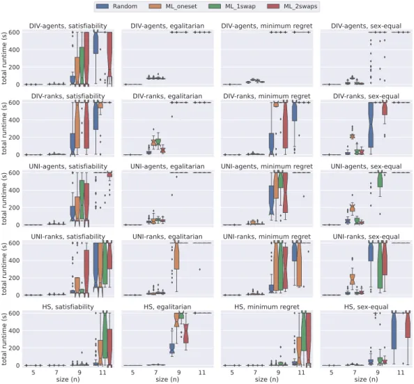
We use notched boxplots [36] in Figures 1, 2, 3, and 4. Figure 1 presents a comparison of total time required by all five models on instances of size 5≤n≤11 under weak stability solved using Gecode. The first insight gained is that thehs model handles the instances of small sizes very well. When we examine performance based on the dataset generation methods, we observe that usually a weakly stable matching for the instances in Random is found faster than other datasets when using Gecode. Additionally we observe that the

(11)

0 200 400 600

total runtime (s)

DIV-agents, satisfiability DIV-agents, egalitarian DIV-agents, minimum regret DIV-agents, sex-equal

0 200 400 600

total runtime (s)

DIV-ranks, satisfiability DIV-ranks, egalitarian DIV-ranks, minimum regret DIV-ranks, sex-equal

0 200 400 600

total runtime (s)

UNI-agents, satisfiability UNI-agents, egalitarian UNI-agents, minimum regret UNI-agents, sex-equal

0 200 400 600

total runtime (s)

UNI-ranks, satisfiability UNI-ranks, egalitarian UNI-ranks, minimum regret UNI-ranks, sex-equal

5 7 9 11

size (n) 0

200 400 600

total runtime (s)

HS, satisfiability

5 7 9 11

size (n) HS, egalitarian

5 7 9 11

size (n) HS, minimum regret

5 7 9 11

size (n) HS, sex-equal Random ML_oneset ML_1swap ML_2swaps

Figure 1A comparison of total time spent by all models under weak stability using Gecode.

models require more time to solve the instances in ML_1swap for satisfiability, egalitarian, and minimum regret versions. On the other hand, for the sex-equal version of the problem, ML_oneset is the most challenging dataset for all models. We conclude from this figure that hsis the best model when dealing with small instances under weak stability using Gecode.

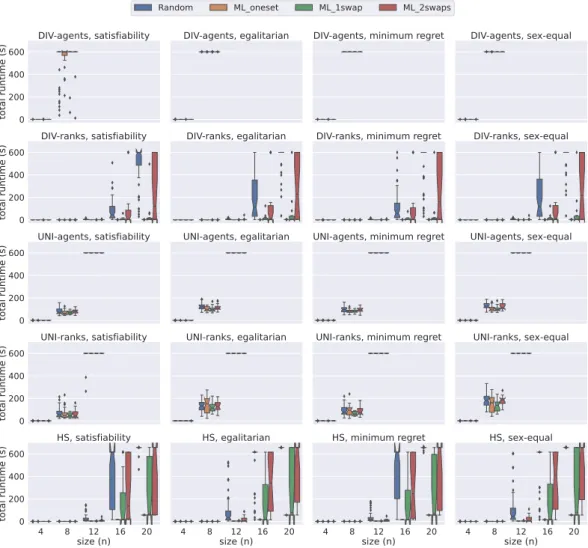
Figure 2 demonstrates the results obtained from the same datasets under strong stability.

Note that the problem model for finding a matching under weak stability is a relaxed version of the model under strong stability. However, it is interesting to observe from the experiments that, on average, strongly stable matchings are found faster than their weak counterpart.

We can clearly observe this behaviour on Figure 2. All models except div-agents were able to solve all satisfiable instances of size between 4 ≤ n ≤ 11 within the given time limit. Therefore, in order to provide more insight into the performance of models, we use a larger scale, i.e.{4,8,12,16,20}in Figure 2. Under strong stability, we clearly observe that hs anddiv-ranks scale better when compared to the other models. For instance, for the satisfiability problem with sizen= 8, both hsanddiv-ranks quickly solve all the instances.

However, bothuni-agents anduni-ranks require longer time thanhsanddiv-ranks, whereas div-agents fails to solve many instances within the given time-limit. Bothuniandhsfollow the same commitment approach (group commitment). We believe this is hampering their

(12)

0 200 400 600

total runtime (s)

0 200 400 600

total runtime (s)

0 200 400 600

total runtime (s)

0 200 400 600

total runtime (s)

UNI-ranks, satisfiability UNI-ranks, egalitarian UNI-ranks, minimum regret UNI-ranks, sex-equal

4 8 12 16 20

size (n) 0

200 400 600

total runtime (s)

HS, satisfiability

4 8 12 16 20

size (n) HS, egalitarian

4 8 12 16 20

size (n) HS, minimum regret

4 8 12 16 20

size (n) HS, sex-equal Random ML_oneset ML_1swap ML_2swaps

Figure 2A comparison of total time spent by all models under strong stability using Gecode.

scalability as there are fewer solutions in the strong stability case, which increases the chances of making wrong choices thus leading to higher penalties in the case of group commitment as we have to undo the three pairings. Considering that the time performance ofunimodels anddiv-agents are considerably worse for 4≤n≤12 when compared to others, we decided to discard them from further experiments. hsis not performing that bad, but its scalability is affected by the computation of the BT sets. The size of each BT set isO(n³), which is a remarkable overhead when dealing with big instances. We elaborate more on this limitation in the next section. Therefore, we conclude from this figure thatdiv-ranks is the most efficient model when working with largenunder strong stability using Gecode.

Note thathswas implemented in Gecode directly because it is cheaper to carry out the computation of the BT sets in C++ than in MiniZinc. However, this decision does not put the other models in a disadvantageous position since the main contribution to the running time comes from the solving time and in all cases the solving phase is carried out in C++.

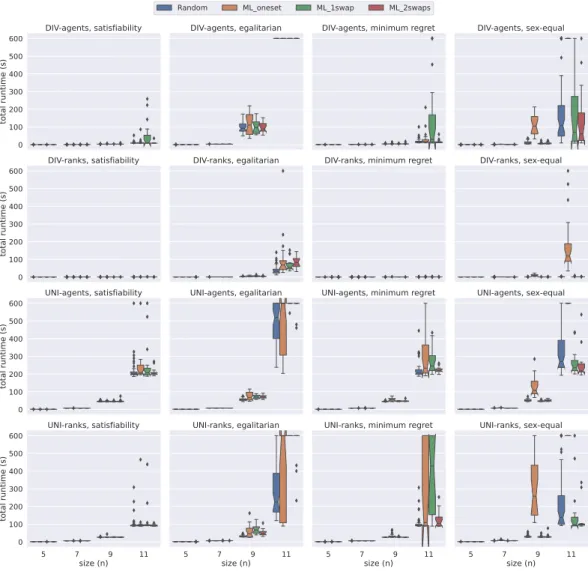
In addition to the Gecode experiments, we tested our four modelsdiv-agents,div-ranks, uni-agents, and uni-ranks on Chuffed. Chuffed is the state-of-the art lazy clause solver that performs propagation by recording the reasons of propagation at each step. This helps with efficiently creating nogoods during the search and avoiding failures. Note that due to

(13)

0 100 200 300 400 500 600

total runtime (s)

0 100 200 300 400 500 600

total runtime (s)

0 100 200 300 400 500 600

total runtime (s)

5 7 9 11

size (n) 0

100 200 300 400 500 600

total runtime (s)

UNI-ranks, satisfiability

5 7 9 11

size (n) UNI-ranks, egalitarian

5 7 9 11

size (n) UNI-ranks, minimum regret

5 7 9 11

size (n) UNI-ranks, sex-equal Random ML_oneset ML_1swap ML_2swaps

Figure 3A comparison of total time spent by all models excepthsunder weak stability using Chuffed.

implementing thehsmodel directly in Gecode, our Chuffed experiment results do not include the performance of thehsmodel. Figure 3 presents a comparison of div-agents,div-ranks, uni-agents, and uni-ranks models on instances of size 5≤n≤11 under weak stability. In these plots, we can clearly observe thatdiv-ranks model has an advantage over the others in terms of total time required to complete the experiments. It is interesting to observe that contrasting with the findings of Gecode experiments in Figure 1, wherediv-agents seems to have an analogous performance with div-ranks, if not better, we observe in Figure 3 thatdiv-ranks has a clear advantage overdiv-agents when using Chuffed. We believe this shows thatdiv-ranks benefits greatly from nogood learning. Additionally, using Figure 3, we can verify our previous observation about ML_oneset being a more challenging dataset generation method for the sex-equal variant under weak stability.

Lastly, Figure 4 demonstrates a comparison of div-agents,div-ranks,uni-agents, anduni- ranks models on instances of size 5≤n≤11 under strong stability. A very straightforward intuition of these tests is that theuni-agents anduni-ranks models are not able to scale well to larger instances. On the other hand, we observe thatdiv-agents handles an increase in

(14)

0 100 200 300 400

total runtime (s)

0 100 200 300 400

total runtime (s)

0 100 200 300 400

total runtime (s)

5 7 9 11

size (n) 0

100 200 300 400

total runtime (s)

UNI-ranks, satisfiability

5 7 9 11

size (n) UNI-ranks, egalitarian

5 7 9 11

size (n) UNI-ranks, minimum regret

5 7 9 11

size (n) UNI-ranks, sex-equal Random ML_oneset ML_1swap ML_2swaps

Figure 4A comparison of total time spent by all models excepthsunder strong stability using Chuffed.

the number of agents better than theuni models, but it still performs worse thandiv-ranks whenn≥9. Considering the stable and rapid performance of div-ranks using Chuffed and also combining this with our observation on Figure 2, we conclude that thediv-ranks model is the best one to solve3dsm-cycunder strong stability.

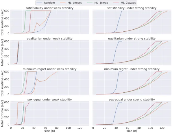
4.3 Scalability

Consideringdiv-ranks is the best performing model in the majority of cases, we performed further experiments using this model on instances withn∈ {20,23,26,29,32,35,40,45,50,60, 70,80,90,100,110,120,130}.

Figure 5 presents a comparison of the median total time required by div-ranks using failmin strategy on all four datasets both under weak and strong stability. An interesting insight from this figure is that all four problem variants (i.e. satisfiability, egalitarian, minimum regret, and sex-equal) result in similar performances under strong stability, where instances in Random require the longest time to be solved and ML_oneset requires the least. However,

(15)

0 200 400 600

total runtime (sec)

satisfiability under weak stability satisfiability under strong stability

0 200 400 600

total runtime (sec)

egalitarian under weak stability egalitarian under strong stability

0 200 400 600

total runtime (sec)

minimum regret under weak stability minimum regret under strong stability

0 20 40 60 80 100 120

size (n) 0

200 400 600

total runtime (sec)

sex-equal under weak stability

0 20 40 60 80 100 120

size (n)

sex-equal under strong stability Random ML_oneset ML_1swap ML_2swaps

Figure 5An overview of the performance ofdiv-ranks using Chuffed under both weak and strong stability when solving problem instances of different sizes for each dataset.

we cannot make such a generalisation for weakly stable matchings. For instance, ML_oneset dataset is the most challenging dataset for the sex-equal problem variant, but it is also the least challenging for the minimum regret variant under weak stability.

5 Conclusion and future work

We proposed a collection of Constraint Programming models to solve the 3-dimensional stable matching problem with cyclic preferences (3dsm-cyc) using both strong and weak stability notions. Additionally, we extended some well-known fairness notions (egalitarian, minimum regret, and sex-equal) to3dsm-cyc. The five proposed models are fundamentally different from each other in terms of their commitment (individual or group), and also their domain values (agents or ranks). Our experiments show that nogood learning benefits some models more than others. An unexpected observation is that strong stability turns out to be easier to solve than weak stability. Following a comprehensive empirical evaluation, we conclude that the performances of the proposed models differ with respect to the type of stability and dataset generation method.

The models proposed can be easily adapted to take advantage of the good performance of strong stability by first trying to find a strongly stable matching. Other future work could extend our models to more types of instances, for example by allowing preference lists to be incomplete. One could also look at other redundant constraints in order to best take

(16)

advantage of the properties that some instances exhibit with regard to fairness objectives.

We remarked thathspays a high price for the generation of the BT sets but it is possible to generate the sets by demand instead of doing it eagerly.

References

1 D. J. Abraham, A. Levavi, D. F. Manlove, and G. O’Malley. The stable roommates problem with globally-ranked pairs. Internet Mathematics, 5:493–515, 2008.

2 Ahmet Alkan. Nonexistence of stable threesome matchings. Mathematical Social Sci- ences, 16(2):207–209, 1988. URL:https://www.sciencedirect.com/science/article/pii/

0165489688900534.

3 Michel Balinski and Tayfun Sönmez. A tale of two mechanisms: Student placement. Journal of Economic Theory, 84(1):73–94, 1999. URL:https://www.sciencedirect.com/science/

article/pii/S0022053198924693.

4 Péter Biró, Robert W Irving, and Ildikó Schlotter. Stable matching with couples: An empirical study. Journal of Experimental Algorithmics (JEA), 16:Article no. 1.2, 2011.

5 Péter Biró and Eric McDermid. Three-sided stable matchings with cyclic preferences. Al- gorithmica, 58(1):5–18, 2010. doi:10.1007/s00453-009-9315-2.

6 Endre Boros, Vladimir Gurvich, Steven Jaslar, and Daniel Krasner. Stable matchings in three-sided systems with cyclic preferences.Discret. Math., 289(1-3):1–10, 2004. doi:10.1016/

j.disc.2004.08.012.

7 Sebastian Braun, Nadja Dwenger, and Dorothea Kübler. Telling the truth may not pay off:

An empirical study of centralized university admissions in Germany. The B.E. Journal of Economic Analysis and Policy, 10, article 22, 2010.

8 Yan Chen and Tayfun Sönmez. Improving efficiency of on-campus housing: an experimental study. American Economic Review, 92:1669–1686, 2002.

9 Geoffrey Chu.Improving combinatorial optimization. PhD thesis, University of Melbourne, Australia, 2011. URL:http://hdl.handle.net/11343/36679.

10 Sofie De Clercq, Steven Schockaert, Martine De Cock, and Ann Nowé. Solving stable matching problems using answer set programming.Theory Pract. Log. Program., 16(3):247–268, 2016.

doi:10.1017/S147106841600003X.

11 Lin Cui and Weijia Jia. Cyclic stable matching for three-sided networking services.Comput.

Networks, 57(1):351–363, 2013. doi:10.1016/j.comnet.2012.09.021.

12 Vladimir I. Danilov. Existence of stable matchings in some three-sided systems. Math. Soc.

Sci., 46(2):145–148, 2003. doi:10.1016/S0165-4896(03)00073-8.

13 Joanna Drummond, Andrew Perrault, and Fahiem Bacchus. SAT is an effective and complete method for solving stable matching problems with couples. InProceedings of the Twenty-Fourth International Joint Conference on Artificial Intelligence, IJCAI 2015, Buenos Aires, Argentina, July 25-31, 2015, pages 518–525. AAAI Press, 2015. URL:http://ijcai.org/Abstract/15/

079.

14 Pavlos Eirinakis, Dimitris Magos, Ioannis Mourtos, and Panayiotis Miliotis. Finding all stable pairs and solutions to the many-to-many stable matching problem. INFORMS J. Comput., 24(2):245–259, 2012. doi:10.1287/ijoc.1110.0449.

15 Kimmo Eriksson, Jonas Sjöstrand, and Pontus Strimling. Three-dimensional stable matching with cyclic preferences. Math. Soc. Sci., 52(1):77–87, 2006. doi:10.1016/j.mathsocsci.2006.

03.005.

16 Guillaume Escamocher and Barry O’Sullivan. Three-dimensional matching instances are rich in stable matchings. InIntegration of Constraint Programming, Artificial Intelligence, and Operations Research - 15th International Conference, CPAIOR 2018, Delft, The Netherlands, June 26-29, 2018, Proceedings, volume 10848, pages 182–197. Springer, 2018. doi:10.1007/

978-3-319-93031-2_13.