MŰHELYTANULMÁNYOK DISCUSSION PAPERS
INSTITUTE OF ECONOMICS, CENTRE FOR ECONOMIC AND REGIONAL STUDIES, HUNGARIAN ACADEMY OF SCIENCES - BUDAPEST, 2018
MT-DP – 2018/20
Paths to stable allocations
ÁGNES CSEH – MARTIN SKUTELLA
2
Discussion papers MT-DP – 2018/20
Institute of Economics, Centre for Economic and Regional Studies, Hungarian Academy of Sciences
KTI/IE Discussion Papers are circulated to promote discussion and provoque comments.
Any references to discussion papers should clearly state that the paper is preliminary.
Materials published in this series may subject to further publication.
Paths to stable allocations
Authors:
Ágnes Cseh research fellow
Hungarian Academy of Sciences, Centre for Economic and Regional Studies, Institute of Economics
E-mail: cseh.agnes@krtk.mta.hu
Martin Skutella
Einstein-Professor für Mathematik und Informatik TU Berlin, Institut für Mathematik, Germany
E-mail: skutella@math.tu-berlin.de
August 2018
3
Paths to stable allocations Ágnes Cseh – Martin Skutella
Abstract
The stable allocation problem is one of the broadest extensions of the well-known stable marriage problem. In an allocation problem, edges of a bipartite graph have capacities and vertices have quotas to fill. Here we investigate the case of uncoordinated processes in stable allocation instances. In this setting, a feasible allocation is given and the aim is to reach a stable allocation by raising the value of the allocation along blocking edges and reducing it on worse edges if needed. Do such myopic changes lead to a stable solution?
In our present work, we analyze both better and best response dynamics from an algorithmic point of view. With the help of two deterministic algorithms we show that random procedures reach a stable solution with probability one for all rational input data in both cases. Surprisingly, while there is a polynomial path to stability when better response strategies are played (even for irrational input data), the more intuitive best response steps may require exponential time. We also study the special case of correlated markets. There, random best response strategies lead to a stable allocation in expected polynomial time.
Keywords: stable matching, stable allocation, paths to stability, best response strategy, better response strategy, correlated market
JEL Classification: C63, C78 Acknowledgement:
A short version of this paper has appeared in the proceedings of SAGT 2014, the 7th
International Symposium on Algorithmic Game Theory. Cseh was supported by OTKA grant
K128611, the Hungarian Academy of Sciences (KEP-6/2017), its Momentum Programme
(LP2016-3/2016) and its János Bolyai Research Fellowship.
4
Stabil allokációkhoz vezető utak Cseh Ágnes – Martin Skutella
Összefoglaló
A stabil allokációprobléma a stabil párosításprobléma egy általánosítása.
Egy allokációproblémában az adott páros gráf élein kapacitások, csúcsain pedig kvóták találhatók. Cikkünkben a központi koordináció nélküli folyamatokat vizsgáljuk. Ebben a kérdéskörben egy megengedett allokáció adott és a cél az, hogy blokkoló élek kielégítésével stabilizáljuk ezt az allokációt. Fő kérdésünk az, hogy ilyen változásokkal eljuthatunk-e egy valóban stabil megoldáshoz.
Mind a jobb, mind a legjobb lépések módszerét tanulmányozzuk cikkünkben.
Két determinisztikus algoritmus segítségével megmutatjuk, hogy egy valószínűséggel ér el mindkét fent említett folyamat stabil megoldást. Meglepő módon a jobb lépések módszerének esetében létezik polinomiális hosszú út a stabilitáshoz, míg a kézenfekvőbb legjobb lépések módszere exponenciálisan hosszú is lehet. Tanulmányozzuk az összefüggő piacok esetét is, ahol várható polinomiális időben konvergál stabil megoldáshoz a legjobb lépések módszere.
Tárgyszavak: stabil párosítás, stabil allokáció, út a stabilitáshoz, legjobb lépések módszere, jobb lépések módszere, összefüggő piacok
JEL: C63, C78
Ágnes Cseh · Martin Skutella
Abstract The stable allocation problem is one of the broadest extensions of the well-known stable marriage problem. In an allocation problem, edges of a bipartite graph have capacities and vertices have quotas to fill. Here we in- vestigate the case of uncoordinated processes in stable allocation instances. In this setting, a feasible allocation is given and the aim is to reach a stable allo- cation by raising the value of the allocation along blocking edges and reducing it on worse edges if needed. Do such myopic changes lead to a stable solution?
In our present work, we analyze both better and best response dynamics from an algorithmic point of view. With the help of two deterministic algo- rithms we show that random procedures reach a stable solution with proba- bility one for all rational input data in both cases. Surprisingly, while there is a polynomial path to stability when better response strategies are played (even for irrational input data), the more intuitive best response steps may require exponential time. We also study the special case of correlated markets.
There, random best response strategies lead to a stable allocation in expected polynomial time.
Keywords stable matching · stable allocation · paths to stability · best response strategy·better response strategy·correlated market
A short version of this paper has appeared in the proceedings of SAGT 2014, the 7th In- ternational Symposium on Algorithmic Game Theory. Cseh was supported by OTKA grant K128611, the Hungarian Academy of Sciences (KEP-6/2017), its Momentum Programme (LP2016-3/2016) and its János Bolyai Research Fellowship.
Á. Cseh
Hungarian Academy of Sciences, Centre for Economic and Regional Studies, Institute of Economics, Tóth Kálmán u. 4., 1097 Budapest, Hungary
Tel.: +36-1-224-6700
E-mail: cseh.agnes@krtk.mta.hu M. Skutella
TU Berlin, Institut für Mathematik, Straße des 17. Juni 136, 10623 Berlin, Germany E-mail: skutella@math.tu-berlin.de
1 Introduction
Capacitated matching markets without prices model various real-life problems such as, e. g., employee placement, task scheduling or admission procedures.
Research on those markets focuses on maximizing social welfare instead of profit. Stability is probably the most widely used optimality criterion in that case.
Finding equilibria in markets that lack a central authority of control is an- other widely studied, challenging task. Besides modeling uncoordinated mar- kets such as third-generation (3G) wireless data networks [11] and ride-sharing systems [18], selfish and uncontrolled agents can also represent modifications in coordinated markets, e. g., the arrival of a new agent or slightly changed preferences [4]. In our present work, those two topics are combined: we study uncoordinated capacitated matching markets.
1.1 Stability in matching markets
The theory of stable matchings has been investigated for decades. Gale and Shapley [10] introduced the notion of stability on their well-knownstable mar- riage problem. An instance of this problem consists of a bipartite graph where the two vertex groups symbolize men and women, respectively. Each agent has a preference list of their acquaintances of the opposite gender. A set of marriages (a matching) isstable, if no pair blocks it. Ablocking pairis an un- married pair so that the man is single or he prefers the woman to his current wife and vice versa, the woman is single or she prefers the man to her current husband. The Gale-Shapley algorithm was the first proof for the existence of stable matchings.
A natural extension of matching problems arises when capacities are in- troduced. The stable allocation problem is defined in a bipartite graph with edge capacities and quotas on vertices. The exact problem formulation and a detailed example are provided in Section 2.
1.2 Better and best response steps in uncoordinated markets
Central planning is needed in order to produce a stable solution with the Gale- Shapley algorithm. In many real-life situations, however, such a coordination is not available. Yet stability is a naturally desirable property of uncoordinated markets. A stable matching seems to be the best reachable solution for all agents, because they cannot find any partnership that could improve their own position. In uncoordinated markets, agents play their selfish strategy, trying to reach the best possible solution.
Apath to stabilityis a series of myopic operations, each of which can occur without any central coordination. The intuitive picture of a myopic operation is the following. If a man and a woman block a marriage scheme, then they
j3
j2
j1
m1 m2 m3
3
1 1
2 2
1 1
3
2
1 3
2 2
2
3
3
1
3
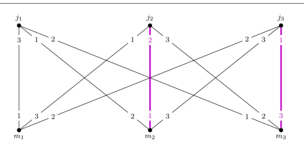
Fig. 1 A stable marriage instance and a cycle of best response blocking edges. Starting with the unstable matching (j2m2, j3m3), and saturating the blocking edgesj1m3,j2m1, j3m1,j1m2,j2m2,j3m3 in this order leads back to the same unstable matching. In each round, the chosen blocking edge is the best blocking edge of the corresponding vertexji.
both agree to form a couple together, even if they divorce their current partners to that end. The recently divorced agents may induce new blocking pairs. In a path to stability, such changes are made until a stable matching is reached.
The study of uncoordinated matching processes has a long history. In the case of one-to-one matchings, two different concepts have been studied:
better and best response dynamics. One of the agent groups is chosen to be the active side. These vertices submit proposals to the passive vertices. Ac- cording tobest response dynamics, the best blocking edge of an active vertex is chosen to perform myopic changes along. In better response dynamics, any blocking edge can play this role. Observe that the Gale-Shapley algorithm it- self can be seen as series of best response steps, with men being the active side.
The core questions regarding uncoordinated processes rise naturally. Can a series of myopic changes result in returning back to the same unstable match- ing? If yes, is there a way to reach a stable solution? How do random procedures behave? The first question about uncoordinated two-sided matching markets was brought up by Knuth [15] in 1976. He also gives an example of a match- ing problem where better response dynamics cycle. More than a decade later, Roth and Vande Vate [17] came up with the next result on the topic. They show that random better response dynamics converge to a stable matching with probability one. Analogous results for best response dynamics were pub- lished in 2011 by Ackermann et al. [2]. They also show an instance in which best response dynamics cycle (see Figure 1), give a deterministic algorithm for reaching a stable solution in polynomial time and prove that the convergence time is exponential in both random cases.
Besides these works on the classical stable marriage problem, there is a number of papers investigating variants of it from the paths-to-stability point of view. For the stable roommates problem, the non-bipartite version of the stable marriage problem, it is known that there is a series of myopic operations
that leads to a stable solution, if one exists [7]. A path to stability also exists in the bipartite matching case with payments where flexible salaries and produc- tivity are taken into account [5]. In the hospitals/residents assignment problem with couples, the existence of such a path is only guaranteed if the preferences are weakly responsive [14]. Weak responsiveness ensures consistence between the preferences of each partner and the couple’s preference list on pairs of hospitals. In many-to-many markets, supposing substitutable preferences on one side and responsive preferences on the other side, a path to stability can be found [16]. Both substitutable and responsive preferences are defined in instances where preferences are given on sets of vertices. In the case of one-to- one bipartite matching markets, closely related optimality concepts, such as socially stable, locally stable, friendship matching, and considerate matching have also been investigated in uncoordinated markets [13]. Although many variants of the stable marriage problem have been studied, no paper discusses the case of allocations (instead of matchings orb-matchings), where edges are capacitated, and thus, might be partially contained in stable solutions. Our present work makes an attempt to fill this gap in the literature.
Structure of the paper In the next section, the essential theoretical basis is pro- vided: besides stable allocations, better and best response modifications are also defined formally. In Section 3, allocation instances with characteristic pref- erence profiles are investigated. We show that although random best response processes generally run in exponential time, in the case of correlated markets, polynomial convergence is expected. Better and best response dynamics in the general case on rational input are extensively studied in Section 4. We describe two deterministic algorithms that generalize the result of Ackermann et al. on one-to-one matching markets to stable allocation instances and also show algorithmic differences between better and best response strategies. In the case of random procedures, convergence is shown for both strategies. Sec- tion 5 focuses on running time efficiency and contains our main result. There, a better response algorithm is presented that terminates with a stable solution in O(|V|2|E|) time in a graph with |V| vertices and|E| edges, even for irra- tional input data. A counterexample proves that such an acceleration cannot be reached for the best response dynamics. Our contribution is summarized in Table 1.
shortest path to stability random path to stability best response dynamics exponential length converges with probability 1 better response dynamics polynomial length converges with probability 1 Table 1 Our results for a shortest and a random path to a stable allocation in instances with rational input.
Applied to a matching instance, our best-response algorithm (in Section 4) performs the same steps as the two-phase best response algorithm of Acker- mann et al. Our better-response variant can also be interpreted as an extended
version of the above mentioned method. The only difference is that while our first phase is better response, while theirs is best response. However, this seems to be a minor difference, as their proof is also valid for a better response first phase, and our proof still holds if only best blocking edges are chosen.
Moreover, stable allocations might be the most complex model in which this approach brings results. The most intuitive extension of Ackermann et al.’s al- gorithm for stable flows, defined by Fleiner [8], does not even result in feasible myopic changes.
On the other hand, our accelerated better-response algorithm (in Section 5) generalizes another known method, the polynomial algorithm that finds a sta- ble allocation. Applied directly to an instance with empty allocation, our accel- erated Phase II performs augmentations like the augmenting path algorithms of Baïou and Balinski [3], and of Dean and Munshi [6]. Since our acceler- ated Phase II is a slightly modified variant of our first algorithm, our solution concept offers a bridge between two known methods for solving two different problems, namely the paths to stability problem in stable marriage instances and the stable allocation problem, providing a solution to both of them.
2 Preliminaries
In this section we define stable allocations formally, and then proceed to the description of better and best response myopic changes in stable allocation instances.
2.1 Stable allocations
The stable marriage problem has been extended in several directions. A great deal of research effort has been spent on many-to-one and many-to-many matchings, sometimes also referred to asb-matchings. Their extension is called thestable allocation problem, also known as the ordinal transportation prob- lem, since it is a direct analog of the classical cost-based transportation prob- lem. In this problem, the vertices of a bipartite graph G= (V, E) havequo- tas q : V(G) → R≥0, while edges have capacities c : E(G) → R≥0. Both functions arereal-valued, unlike the respective functions in many-to-many in- stances, where capacities are unit, while quotas are integer-valued. Therefore, allocations can model more complex problems, for example where goods can be divided unequally between agents. In order to avoid confusion caused by terms associated with the marriage model, we call the vertices of the first side jobs and the remaining verticesmachines. For each machine, its quota is the maximal time spent working. A job’s quota is the total time that machines must spend on the job in order to complete it. In addition, machines have a limit on the time spent on a specific job; this is modeled by edge capacities.
A feasible allocation is a set of contracts where no machine is overloaded and no job is worked on after it has been completed.
Definition 1 (allocation) Functionx:E(G)→R≥0 is called anallocation if for every edgee∈E(G) and every vertexv∈V(G):
1. x(e)≤c(e);
2. x(v) :=P
e∈δ(v)x(e)≤q(v), where δ(v) is the set of edges incident tov.
For an edge e with x(e) > 0 we say that e is in x. To define stability we needpreference listsas well. All vertices rank their incident edges strictly.
Vertex v prefersuv to wv, if uv is ranked better on v’s preference list than wv: rankv(uv)<rankv(wv). In this case we say that uv dominates wv at v.
A stable allocation instance consists of four elements: (G, q, c, O), where O is the set of all preference lists.
Definition 2 (blocking edge, stable allocation)An allocationxisblocked by an edgejmif all of the following properties hold:
1. x(jm)< c(jm);
2. x(j)< q(j) orj prefersjmto its worst edge with positive value inx;
3. x(m)< q(m) ormprefersjmto its worst edge with positive value inx.
A feasible allocation isstableif no edge blocks it.
In other words, edge jm is blocking if it is unsaturated and neither end vertices ofjmhas filled up its quota with at least as good edges asjm. If an unsaturated edge fulfills the second criterion, then we say that itdominates x at j. Similarly, if the third criterion is fulfilled for an unsaturated edge, then we talk about an edge dominatingxat m.
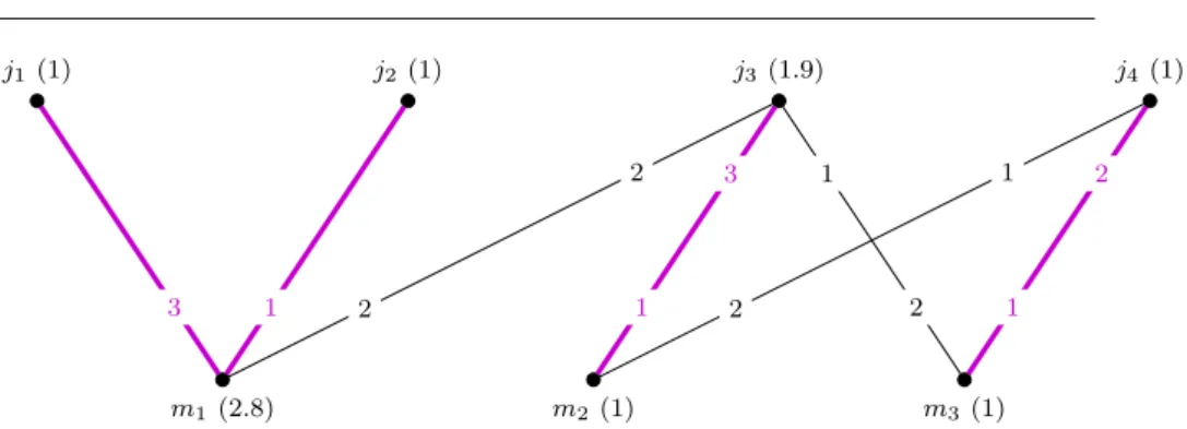
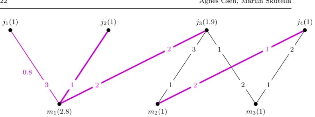
Example 1 Figure 2 illustrates a stable allocation instance. We use the same example throughout the entire paper to demonstrate different notions defined here. For the sake of simplicity, all edge capacities are unit. The numbers within parenthesis over and under the vertices represent the quota function.
The preferences can be seen on the edges: the more preferred edges carry a better rank, i.e., a smaller number. For example, machinem1’s most preferred job isj2, its second choice isj3, while its least preferred, but still acceptable job isj1. The functionx= 1 on the colored edges andx= 0 on the remaining edges is a feasible allocation, since no quota or capacity constraint is violated. The unique blocking edge is easy to find:j3m1blocksx, because it is unsaturated and both end vertices have free quota.
Baïou and Balinski [3] prove that stable allocations always exist. They also give two algorithms for finding them, an extended version of the Gale-Shapley algorithm and an inductive algorithm. The worst case running time of the first algorithm is exponential, but the latter one runs in strongly polynomial time.
Dean and Munshi [6] speed up the polynomial algorithm using sophisticated data structures: their version runs in O(|E|log|V|) time for any real-valued instance.
j3(1.9) j4(1) j2 (1)
j1 (1)
m1(2.8) m2(1) m3(1)
2
2
1
2 3
1
1
2
2
1 1
3
Fig. 2 A stable allocation instance with unit capacities and a feasible, but unstable alloca- tion, marked by colored edges.
2.2 Better and best response steps for allocations
First, we provide some basic definitions and notations we will use throughout the entire paper. A feasible, but possibly unstable allocationxis given at the beginning, thus the instance can be written as I= (G, q, c, O, x). In our in- stanceI, jobs form the active sideJ, while machinesM are passive players.
For the sake of simplicity we denote the residual capacity c(jm)−x(jm) of edge jm by ¯x(jm) and similarly, the residual quota q(v)−x(v) of vertex v by ¯x(v). The definition of better and best response strategies is not as straight- forward as it is in the matching instance with unit quotas and capacities. Here, the possible outcomes for a player are ordered lexicographically. We say that machinem prefers allocationx1 to allocationx2 ifx1(j0m)> x2(j0m) the for the best ranked edgej0mamong edges withx1(jm)6=x2(jm).
Although lexicographic order seems to be a natural choice, it is somewhat against the convention when discussing stable allocations. In most cases, when comparing the position of an agent in two stable allocations, the so calledmin- min criterionis used [3]. According to this rule, the agent prefers the allocation in which its worst edge in x is ranked better. In order to make use of such an ordering relation, each vertex has to have the same allocation value in all stable solutions. Therefore here, when studying and comparing arbitrary feasible allocations, this concept proves to be counter-intuitive.
An active playerj having some blocking edges is chosen to perform abest response step on the current allocationx. Amongstj’s blocking edges, letjm be the one ranked best on j’s preference list. The aim of playerj is to reach its best possible lexicographic position via increasingx(jm). To this end,j is ready to allocate all its remaining quota ¯x(j) tojm, moreover, it may reassign allocation from all edges worse thanjmtojm. Thus,jaims to increasex(jm) by ¯x(j) +x(edges dominated byjm atj). To preserve feasibility,x(jm) is not increased by more than ¯x(jm). The passive playermagrees to increasex(jm) as long as it does not lose allocation on better edges. This constraint gives the third upper bound, ¯x(m) +x(edges dominated byjmat m). To summarize this, in a best response stepx(jm) is increased by the following amount.
A:= min{x(j) +¯ x(edges dominated byjmatj),x(jm),¯
¯
x(m) +x(edges dominated byjm atm)}
Once this A and the new x(jm) is determined,j and m fill their remaining quota, then refuse allocation on their worst allocated edges, until xbecomes feasible.
Better response steps are much less complicated to describe. The chosen active vertexjincreases the allocation on an arbitrary blocking edgejm. Both j and m are allowed to refuse allocation on worse edges than jm. This rule guarantees that j’s lexicographic situation improves and that the change is myopic for both vertices. By definition, best response steps are always better response steps at the same time. The execution of a single better response step consists of modifications on at most|δ(j)|+|δ(m)| −1≤ |V| −1 edges.
Example 2 In our example above,j3 andm1 mutually agree to allocate value 1 to j3m1. If best response strategies are played, m1 refuses 0.2 amount of allocation from j1m1, while j3 reduces x(j3m2) to 0.9. Through this step, they induce blocking elsewhere inG: nowj4m2 blocks the newx, becausem2
lost some allocation. Thus, another myopic change would now be to increase x(j4m2), and so on. A better response step of the same vertex j3 would be for example to increase x(j3m1) to 1, while refusing j3m2 entirely. To keep feasibility,m1has to refuse 0.2 amount of allocation onj1m1.
3 Correlated markets
Before tackling the general paths to stability problem, we first restrict ourselves to instances with characteristic preference profiles. In this section, we study the case of stable allocations on an uncoordinated market with correlated preferences. Later we will prove that the convergence time of random best and better response strategies is exponential in general instances. By contrast, here we show that on correlated markets, random best response strategies terminate in expected polynomial time, even in the presence of irrational data. At the end of this section we also elaborate on the behavior of better response dynamics.
Definition 3 (correlated market) An allocation instance is correlated, if there is a functionf :E(G)→Nsuch that rankv(uv)<rankv(wv) iff(uv)<
f(wv) for everyu, v, w∈V(G) and no two edges have the same f value.
Correlated markets are also called instances with globally ranked pairs or acyclic markets. The latter property means that there is no cycle of inci- dent edges such that every edge is preferred to the previous one by their common vertex. Abraham et al. [1] show that acyclic markets are correlated and vice versa. The instance depicted in Figure 2 is not correlated: edges (j3m3, j4m3, j4m2, j3m2) form a preference cycle. Ackermann et al. [2] were
the first to prove that random better and best response dynamics reach a stable matching on correlated markets in expected polynomial time. Using a similar argumentation, we extend their result to allocation instances.
Theorem 1 In correlated allocation instances with real-valued input data, random best response dynamics reach a stable solution in expected timeO(|V|2|E|).
Proof Before studying paths to stability we show that in correlated instances, the set of stable solutions has cardinality one. There is an absolute minimum off(jm). The single edgejmwith this minimalf value must be in all stable allocations with value min{c(jm), q(j), q(m)}, otherwise it is blocking. Fixing xonjm and decreasing the quotas of j and mrespectively leads to another correlated allocation instance. In this instance, the stable solutions are ex- actly the stable solutions of the original instance without jm. This leads to an inductive algorithm that proves that there is a unique stable allocation on correlated markets. We now turn to showing that random best response dynamics reach this unique solution in expected polynomial time.
Whenever a job j with an unsaturated edge jm of an absolute mini- mal f(jm) is chosen to submit an offer, its best response strategy is to in- crease x on jm. Due to this single best response operation performed by j, x(jm) = min{c(jm), q(j), q(m)} is reached. The probability that a vertex j ∈ J is chosen to take the next step is at least |J|1 . As mentioned in Sec- tion 2.2, one best response step requires at mostO(|V|) modifications. Thus, in order to reach x(jm) = min{c(jm), q(j), q(m)} on the best edge in G,
|J| · |V| = O(|V|2) modifications are needed in expectation. After this, the edgejmwith minimalf value will have reached its final position in the unique stable allocation. From this point on, x(jm) will never be reduced, because neitherj, nor mhave a better incident edge. Thus,x(jm) can be fixed, and a new minimum off can be chosen for the same procedure as before. The num- ber of iterations is bounded from above by the number of edges in the graph.
The unique stable allocation is thus reached inO(|V|2|E|) time in expectation.
In order to establish a similar result for better response dynamics in real- valued correlated instances, an exact interpretation of random events would be needed. In the matching case, best and better response dynamics differ exclusively in the rank of the chosen blocking edge: when playing best response strategy, the best blocking edge is chosen by an active vertexj. In contrast to this, here, better response steps differ also in the amount of modification and in the edges chosen to refuse allocation along. The first factor indicates a continuous state space.
However, if we assume that any better response step results in reassigning the highest possible allocation value to an arbitrary blocking edge, an analo- gous proof can be derived.
Theorem 2 On correlated allocation instances with real-valued input data, random better response dynamics reach a stable solution in expected timeO(|V|3|E|).
Proof The only difference to the setting with best response steps is that after j is chosen, the expected time of reachingx(jm) = min{c(jm), q(j), q(m)}is larger. In this case,j chooses jmwith probability at least |δ(j)|1 . This implies that reaching the stable allocation value on the best edge takes|δ(j)| ·(|δ(j)|+
|δ(m)| −1) =O(|V|2) steps in expectation. In total, for all verticesj∈J and all edges the algorithm takesO(|V|3|E|) steps in expectation.
4 Best and better responses with rational data
In this section, the case of allocations in an uncoordinated marketwith ratio- nal datais studied. As already mentioned, better and best response dynamics can cycle in such instances. We describe two deterministic methods, a better- response and a best-response algorithm that yield stable allocations in finite time. Our best response algorithm is by definition a better response algorithm as well, yet we present a different, better but not best response strategy in Sec- tion 4.1, because it can be accelerated to reach a stable solution in polynomial time, while the best response strategy cannot, as shown in Section 4.2. The main idea of our algorithms is to distinguish between blocking edges based on the type of blocking at the job: dominance or free quota.
A blocking edge can be of two types. Recall point 2 of Definition 2: if jm blocksx, thenx(j)< q(j) orjprefersjmto its worst edge with positive value inx. We talk aboutblocking of type Iin the latter case, ifjmblocksxbecause j prefersjmto its worst edge having positive value in x. Blocking of type II means thatj has no allocated edge that is worse thanjm, butjhas not filled up its quota yet, x(j)< q(j). Note that the reason of the blocking property atmis not involved when defining the two types.
Example 3 Recall our example in Figure 2. The unique blocking edgej3m1is of type I, becausej3, its active vertex, prefers edgej3m1to its worst allocated edgej3m2.
4.1 Better response dynamics
First, we provide a deterministic algorithm that constructs a finite path to stability from any feasible allocation. In the first phase of our algorithm, only blocking edges of type I are chosen to perform myopic changes along. The ac- tive vertices (jobs) choose one of their blocking edges of type I, not necessarily the best one. In all cases, withdrawal is executed along worst allocated edges.
The amount of new allocation added to the blocking edge is determined in such a way that at least one edge or a vertex becomes saturated or empty.
Thus, in the first phase, active vertices replace their worst edges with better ones, even if they have free quota. When no blocking edge of type I remains, the second phase starts. The allocation value is increased on blocking edges of type II such that they cease to be blocking.
The runtime of our algorithm is exponential. Later, in Section 5 we will show that this algorithm can be accelerated such that a stable solution is reached in strongly polynomial time.
Theorem 3 For every allocation instance with rational data and a given ra- tional feasible allocation x, there is a finite sequence of better responses that leads to a stable allocation.
The main idea of the proof is the following. We need to keep track of the change in the size of the allocation and in the lexicographic position of the active vertices simultaneously. In one step of the first phase along edgejm, ei- ther bothjandmrefuse edges, thus, the size of the allocation|x|=P
j∈Jx(j) decreases, or onlyjdoes so, leaving|x|unchanged and improvingj’s situation lexicographically. Since both procedures are monotone and the second one does not impair the first one, the first phase terminates. Termination of the second phase is implied by the fact that passive vertices improve their lexicographic situation in each step. The technical details of this proof sketch are presented as Claims 4.1 and 4.1.
In the first phase, the jobs propose alongarbitraryblocking edges of type I.
We will show that this process ends with an allocation where no job has a blocking edge of type I. In the second phase, the jobs propose along their best blocking edges of type II. Later we will see that during this phase until termination, no job gets a blocking edge of type I. A pseudocode is provided after the description of both phases.
First phase In one step, an arbitrary blocking edge jm of type I is chosen.
Both end vertices, j and m may refuse some allocation along worse edges when increasing x on jm. Jobj has a refusal pointer r(j) that denotes the worst edge allocated to j, if any exists. Similarly, r(m) stands for the worst currently allocated edge of m. A step of Phase I consists of two or three operations, each alongjm, r(j) and possibly alongr(m). Two operations take place, if m has not filled up its quota yet. In this case, x(r(j)) is decreased byA:= min{x(r(j)),x(jm),¯ x(m)}. At the same time,¯ x(jm) is increased by the same amount. Depending on which expression is the minimal one, edge r(j) becomes empty or jm becomes saturated or m fills up its quota. Note that r(m) plays no role because m does not refuse any allocation. In the remaining case, if m has a full quota, three operations take place, since m has to refuse some allocation. The amount of allocation we deal with is now A := min{x(r(j)),x(jm), x(r(m))}. The allocation on the blocking edge¯ jm will be increased byA, on the other two edges it will be decreased byA, until one of them becomes empty or saturated. We emphasize that whenever a job j with free quota adds a new edge better than its worst allocated edge to x, it withdraws some allocation from the worst edge.
Example 4 We return to our example again. It has already been mentioned that the unique blocking edge j3m1 is of type I. The refusal pointer r(j3)
isj3m2. Sincem1has not filled up its quota yet, its refusal pointerj1m1 is ir- relevant at the moment. Due to the same reason, two operations take place. We augment with the following amount of allocation: min{x(j3m2),x(j¯ 3m1),x(m¯ 1)}= 0.8. After this operation, x(j3m1) = 0.8, x(j3m2) = 0.2, and j3m1 is still a Phase I blocking edge. Since x(m1) =q(m1) holds now, three operations are executed withA= min{x(j3m2),x(j¯ 3m1), x(j1m1)}= 0.2. Nowj3m1is satu- rated, hence it ceases to be blocking. During the first operation,j4m2 became blocking of type I, because m2 lost allocation. In the next step, one unit of allocation is reallocated toj4m2fromj4m3. Butj3m3 then becomes blocking of type I, and so on.
Claim Phase I terminates in finite time.
Proof.We use the following potential function in order to show that the process does not cycle:
Θ(x) :=X
j∈J
X
jm∈E(G)
x(jm) rankj(jm)
Recall that rankj(jm) stands for the rank ofjmonj’s preference list. The smaller rankj(jm) is, the bettermis for j. The expression above is bounded for any feasible allocationx:
0≤Θ(x)≤ |J| · max
jm∈E(G)c(jm)·max
j∈J |δ(j)|.
We will show thatΘ(x) decreases in each step of the procedure. The process terminates if the amount of decrement is always greater than a fixed positive constant. If all data are rational, this is guaranteed.
Considering the potential function, we need to keep track of those two jobs that proposed or got refused, since the allocation of all other jobs remains the same, thus their contributions to the summations ofΘ(x) do not change.
As mentioned above, a step consists of either two or three edges changing their value inx. In the first case, when only two edges change their value inx, there is only one job j that modifies its contribution. Thus Θ(x) decreases, because some allocation will move from a less preferred edge to jm. In the second case, where three edges are involved, there is a jobj that improves its lexicographic position, and another jobj0 that loses allocation. The effect of the first change atj is just as above, Θ(x) decreases. Losing allocation forj0 also decreasesΘ(x), sincex(j0) decreases.
Second phase When the first phase terminates, all blocking edges are of type II.
In the second phase, we are allowed to increase x(j). When improving the allocation along a blocking edgejmof type II,mmay refuse some allocation, butj cannot, since the reason of blocking is thatj has not filled up its quota yet. Thus, we do not need the pointer r(j) any more. One step consists of changes along one edge if x(m)< q(m), or along two edges otherwise. If m has not filled up its quota yet, then we simply assign as much allocation to
j00 j j0
m m0
3 2
2
1 1
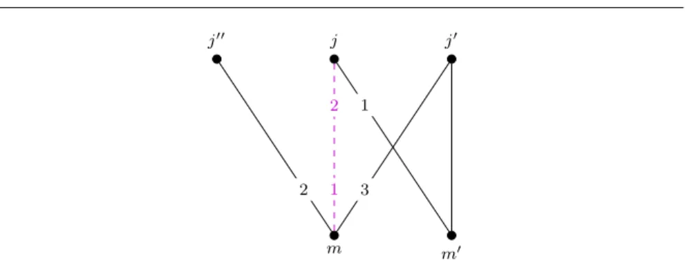
Fig. 3 Edges affected by one myopic operation along the blocking edgejmof type II.
jmas possible withoutx(j), x(m) andx(jm) exceedingq(j), q(m) andc(jm), respectively. If m has to refuse something from a job j0 in order to accept better offers fromj, we improvem’s position untilj0mbecomes empty orjm becomes saturated orj’s quota is filled up.
Claim No step in Phase II can induce a blocking edge of type I.
Proof.One step in Phase II leaves all vertices butj, mand the possibly refused j0unchanged. Thus, if there is a blocking edge of type I after the modification, it must be incident to one of those vertices. The three cases, illustrated in Figure 3, are the following.
– Edge j00m blocks x. The position of m became lexicographically better, thus, no new blocking edge incident to m was introduced. The existing blocking edgesj00mof type II cannot become of type I, becausej00’s position remained unchanged.
– Edgejm0 (orjm) blocksx. The only change at j is thatx(jm) increases, thus,jalso improves its lexicographic position. Therefore, no new blocking edge incident to j appeared. Blocking edges of type II can change their type of blocking only ifjincreased its allocation on a worse edge. But this cannot happen since we chose the best blocking edgejm in Phase II.
– Edge j0m0 (or j0m) blocks x. The only change in j0’s neighborhood is that x(j0m) decreases. After this step, consider an unsaturated edgej0m0 preferred by j0 to its worst allocated edge. Since no machine worsens its lexicographic position in Phase II, ifj0m0 dominates the new allocationx, it already dominated the previous allocation. Therefore, j0m0 must have been a blocking edge of type II prior to the modification and thus remains of type II.
We have argued that once Phase II has started, Phase I can never return.
The last step ahead of us is to show that Phase II may not cycle. But this follows from the fact that in each step exactly one machine strictly improves its lexicographic situation, while all other machines maintain the same allocation as before. In case of a rational input, this improvement is bounded from below, thus, the second phase of the algorithm terminates.
With this we finished the proof of Theorem 3.
Algorithm 1Two-phase better response algorithm
while∃j∈Jwith a blocking edge of type Ido Improvement_I(j)
end while
while∃j∈Jwith a blocking edge of type IIdo Improvement_II(j)
end while
procedureImprovement_I(j) jm←blocking edge of type I ofj if x(m)< q(m)then
A:= min{x(r(j)),¯x(jm),x(m)}¯ x(r(j)) :=x(r(j))−A
x(jm) :=x(jm) +A else
A:= min{x(r(j)),¯x(jm), x(r(m))}
x(r(j)) :=x(r(j))−A x(jm) :=x(jm) +A x(r(m)) :=x(r(m))−A end if
end procedure
procedureImprovement_II(j)
jm←best blocking edge of type II ofj ifx(m)< q(m)then
A:= min{¯x(jm),x(j),¯ x(m)}¯ x(jm) :=x(jm) +A else
A:= min{x(r(m)),x(jm),¯ x(j)}¯ x(jm) :=x(jm) +A
x(r(m)) :=x(r(m))−A end if
end procedure
j1(N) j2(N)
m1(N) m2(N+ 1)
1
2 2
1
1
2
2
1
j1(N+ 1) j2(N)
m1(N) m2(N)
1
2 2
1
1
2
2
1
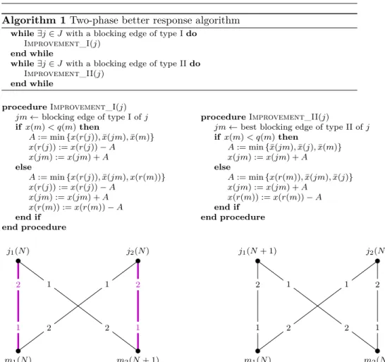
Fig. 4 Worst-case instances for our better response algorithm. On the graph on the left hand-side, Phase I cycles alonghj1m2, j2m2, j2m1, j1m1iN times. In the second instance, Phase II first assignsN amount of allocation to edgesj1m2 andj2m1 and then cyclesN times alonghj1m1, j2m1, j2m2, j1m2i.
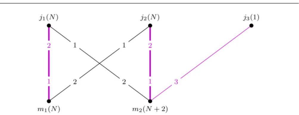
Example 5 The duration of both phases strongly depends on the capacities and quotas. The examples in Figure 4 show two bad instances. The capacity isN on all edges, whereN is an arbitrarily large integer. Quotas are marked above and below the vertices. In the first instance, the initial allocation for Phase I is N on j1m1 and on j2m2 and zero on the remaining two edges.
The first phase performsN augmenting steps along the same cycle. Phase II terminates afterN iterations in the second instance, starting with the empty allocation.
This algorithm also proves an important result regarding rational random better response processes. If the input is rational (there is a smallest positive number that can be represented as a linear combination of all data), it is clearly worthwhile to restrict the set of feasible better response modifications
to the ones that reassign a multiple of this unit. Under this assumption, the set of reachable allocations is finite and they can be seen as states of a discrete time Markov chain. Our algorithm proves that from any state there is a finite path to an absorbing state with a positive probability.
Theorem 4 In the rational case, random better response strategies terminate with a stable allocation with probability one.
Polynomial time convergence cannot be shown for random better response strategies, since they need exponential time to converge in expectation even in matching instances [2].
4.2 Best response dynamics
In this subsection, we derive analogous results for best response modifications to the ones established for better response strategies. The main difference from the algorithmic point of view is that instances can be found in which no series of best response strategies terminates with a stable solution in polynomial time. A simple example shown on the right in Figure 4 resembles the instance given by Baïou and Balinski [3] to prove that the Gale-Shapley algorithm requires exponential time to terminate in stable allocation instances.
Example 6 LetGbe a complete bipartite graph on four vertices, with quota q(j1) =N + 1, (j2) =q(m1) = q(m2) = N, and initial allocation x(j1m1) = x(j2m2) = N for an arbitrary large number N. If the preference profile is chosen to be cyclic, such that rankj1(m1) = rankj2(m2) = rankm1(j2) = rankm2(j1) = 2, the unique series of best response steps consists of 2N opera- tions. This example shows that a polynomial path to stability does not exist, not even for rational input data. A path of exponential length to stability can still be found. Our next theorem shows that this is the case in general.
Theorem 5 For every allocation instance with rational data and a given ra- tional feasible allocation x, there is a finite sequence of best responses that leads to a stable allocation.
Proof Similar to our method for better response strategies, we prove that there is a two-phase algorithm that terminates with a stable solution.
All blocking edges we take into account are best blocking edges of their jobj. Depending on their rank compared toj’s worst allocated edger(j), they are either of type I or type II. A jobj’s best blocking edge jmis
– of type I(a), if rankj(jm)<rankj(r(j)) and
¯
x(j)<min{¯x(jm),x(m) +¯ x(edges dominated byjmatm)};
– of type I(b), if rankj(jm)<rankj(r(j)) and
¯
x(j)≥min{¯x(jm),x(m) +¯ x(edges dominated byjmatm)};
– of type II, if rankj(jm)≥rankj(r(j)).
The intuitive interpretation of the grouping above is given by the steps that we need to execute whenjm is chosen to perform a best response operation.
If jm is of type I(b), then jm can be saturated without any refusal made byj, sincej has sufficient free quota. On the other hand, ifjagrees to reduce x(r(j)) in order to accommodate more allocation onjm, thenjmis a blocking edge of type I(a). The remaining case occurs whenjmis not better thanr(j), that is,j accepts min{x(m),¯ x(j),¯ x(jm)}¯ allocation from m. In this case, no rejection is called byj.
In Phase I, only best blocking edges of type I(a) and I(b) are selected.
Then, when only type II blocking edges remain, Phase II starts. In order to prove finite termination, we introduce two potential functions,Θ(x) andΨ(x).
When proving termination of the first phase, both of them are used, while the second phase is discussed by analyzing the behavior ofΨ(x) only.
The first function Θ(x) comprises two components. The first component is the sum consisting of the rank of refusal pointers at jobs. The second term is a sum consisting of the allocation value of refusal pointers at jobs. When we say thatΘ(x) decreases, it is meant in the lexicographic sense. The second function, Ψ(x) is a set of|M| vectors, each of them corresponding to a ma- chine. Each vector contains|δ(m)|entries, defined asx(jm) for alljm∈δ(m), ordered as they appear in m’s preference list. We denote these vectors by lex(m), because lex(m) increases lexicographically if and only if the lexico- graphic position of mimproves. We added a minus sign in order to keep the terms decreasing. When we say thatΨ(x) decreases we mean that at least one vector in it decreases lexicographically and no vector increases lexicographi- cally. This also implies that we could add up thei-th elements of these vectors and follow the lexicographic increment of the resulting vector. We choose not to do so for intuitive reasons, but the reader can also think ofΨ(x) as a single vector of maxm∈Mdeg(m) scalar components.
Θ(x) := (Θ1(x), Θ2(x)) :=
X
j∈J
rankj(r(j)),X
j∈J
x(r(j))
Ψ(x) :=− lex(m1),lex(m2), ...,lex(m|M|)
Claim The best response step of jobjalong edgejmof type I(a) decreasesΘ(x).
Proof.Due to the type-defining characteristics listed above, there is a rejection on r(j). Ifx(r(j)) becomes 0 through this step, then Θ1(x) decreases, while Θ2(x) might increase. Otherwise, if x(r(j)) > 0 holds even after executing the step, hence Θ1(x) remains unchanged, but Θ2(x) decreases. Any other decrement inx, such as allocation refused bym onr(j0) for somej0 6=j can only further decrease both components ofΘ(x).
Claim The best response step of job j along edgejm of type I(b) decreases Ψ(x) and does not increaseΘ(x).
Proof. Since j does not reject any allocation, x(r(j)) remains unchanged. If any otherr(j0) for somej06=jis affected,Θ(x) is decreased. The only machine whose position changes ismitself: it clearly improves its lexicographic position, thus one component of Ψ(x) decreases, while the remaining vectors remain unchanged.
For any rational input data, the changes inΘ(x) orΨ(x) in each round are bounded from below. Since both functions have an absolute minimum, Phase I terminates in finite time.
Claim The best response step of jobjalong edgejmof type II decreasesΨ(x).
Moreover, no edge becomes blocking of type I(a) or I(b).
Proof. During the second phase, no machine loses allocation, thus, their lexi- cographic position cannot worsen. In addition, for the machine of the current blocking edgejm,lex(m) improves. This also implies that no edgej0m0 dom- inates xat m0 that has not already dominated it before the myopic change.
Moreover, edges that lost allocation during that step are the worst-choice edges of j, hence they cannot be blocking of type I(a) or I(b). If there is an edge j0m0 that became blocking of type I(a) or I(b), then it is better than the worst edge inxatj0. These edges were already unsaturated before the last step and also already dominatedxat both end vertices. This contradicts the fact that best blocking edges are chosen in each step.
The same arguments as above, in Theorem 4, imply the result on random procedures.
Theorem 6 In the rational case, random best response strategies terminate with a stable allocation with probability one.
5 Irrational data – the accelerated algorithm
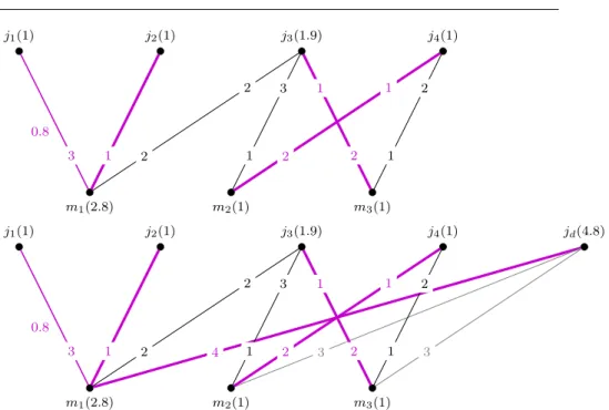
Both of our presented algorithms require exponentially many steps to termi- nate. Moreover, in our previous section we relied several times on the fact that in each step, x is changed with values greater than a specific positive lower bound. When irrational data are present, e.g., q, c orx are real-valued functions, this can no longer be guaranteed. Hence, our arguments for termi- nation are no longer valid. As a matter of fact, some algorithmic ideas do not work with irrational input data, such as in the case of the well-known Ford- Fulkerson algorithm for finding a maximum flow, which fails when irrational capacities are present: the calculated flow might not even converge towards the maximum flow [9, 19]. In this section, we describe a fast version of our two-phase better response algorithm that terminates in polynomial time with a stable allocation for irrational input data as well. We also give a detailed proof of correctness for the first phase and show a construction with which all Phase II steps can be interpreted as Phase I operations in a slightly modified instance.
As usual in graph theory, analternating pathwith respect to an allocation xis a sequence of incident edges that are saturated inxand of those that are unsaturated inxin an alternating manner.
5.1 Accelerated first phase
The algorithm and the proof of its correctness can be outlined in the following way (see also Algorithm 2 below). A helper graph is built in order to keep track of edges that may gain or lose some allocation. A potential function is also defined, which stores information about the structure of the helper graph and the degree of instability of the current allocation. In the helper graph we are looking for paths and cycles to augment along. The amount of allocation we augment with is specified in such a way that the potential function de- creases and the helper graph changes. When using paths and cycles instead of proposal-refusal triplets, more than one myopic operation can be executed at a time. Moreover, we also keep track of consequences of locally myopic improve- ments. For example, we spare running time by avoiding reducing allocation on edges that later become blocking anyway.
First, we elaborate on the structure of the helper graph, define alternating paths and cycles and specify the amount of augmentation. The algorithm, the proof of its correctness, a pseudocode, and an example execution are all described in detail in this section.
Helper graph
Recall that our real-valued input I consists of a stable allocation instance (G, q, c, O) and a feasible allocationx. First, we define a helper graphH(x) on the same vertices asG. This graph is dependent on the current allocation x and will be changed whenever we modifyx. The edge set ofH(x) is partitioned into three disjoint subsets. The first subset P is the set of Phase I blocking edges. Each jobj that has at least one edge with positive xvalue, also has a worst allocated edger(j). When a myopic change is made, jobs tend to reduce xalong exactly these edges. Theserefusal pointers formR, the second subset of E(H(x)). We also keep track of edges that are currently not of blocking type I, but later on they may enter set P. This last subset P0 consists of edges that may become blocking of type I after some myopic changes. An edge jm /∈ P has to fulfill three criteria in order to belong toP0:
1. c(jm)> x(jm);
2. m has at least one refusal edge, i.e.,δ(m)∩ R 6=∅;
3. rankj(jm)<rankj(r(j)).
Such an edge immediately becomes blocking of type I if m loses allocation along one of its refusal edges. Edges inP0 are called possibly blocking edges, the set P ∪ P0 forms the set of proposal edges. Note that a job j may have several edges inP andP0, but at most one inR. Moreover, ifjhas a proposal
edge in H(x), it also has an edge in R. Regarding the machines, if m has a P0-edge, it also has anR-edge. Note that (P ∪ P0)∩ R=∅, because bothP and P0 per definition comprises edges that are ranked better byj thanr(j).
The following lemma provides an additional structural property ofH(x).
Lemma 1 If jm∈ P andj0m∈ P0, then rankm(jm)<rankm(j0m).
That is, blocking edges are preferred to possibly blocking edges by their common machine m.
Proof Since jm ∈ P is a blocking edge of type I, jm dominatesx at m. If the statement is false, then rankm(jm) >rankm(j0m) for some unsaturated edge j0m that is better than the worst allocated edge of j0. Then also j0m dominatesxatm. This, together with the first and last properties of possibly blocking edges implies thatj0m∈ P.
Example 7 Once again we return to our example shown in Figure 2. The only blocking edge j3m1 alone forms P. The set R contains all four edges with positive allocation value: j1m1, j2m1, j3m2 and j4m3. Edges j3m3 and j4m2 are possibly blocking. Thus, in this case,G=H(x).
Alternating paths and cycles
Our algorithm performs augmentations along alternating paths and cycles, so that the allocation value of refusal edges decreases, while the value of proposal edges increases. This is done in such a way thatR,P, orP0(and thus,H(x)) changes. The main idea behind these operations is the same we used in the proof of Theorem 3: reassigning allocation to blocking edges from worse edges, such that the procedure is monotone. The difference between this method and the one presented in Section 4.1 is that, while our first algorithm tackles a single blocking edge in each step, here we deal with several blocking edges (forming the alternating path or cycle) at once.
When constructing the alternating proposal-refusal path or cycleρto aug- ment along, the following rules have to be obeyed:
1. The first edgej1m1 is aP-edge and it is the best proposal edge ofm1. 2. P and P0-edges are added to ρ together with the refusal edge they are
incident with on the active side.
3. Machines choose their bestP orP0-edge.
4. Walkρends atmif
(i) mhas no proposal edge or
(ii) ρreturns to its starting vertex, that is,m=m1 or
(iii) m’s best proposal edge runs to a job already visited byρor
(iv) m’s best proposal edge runs to a job whose refusal pointer points to a machine already onρ.
As long as there is a blocking edge of type I, the first edge j1m1 of such a path or cycle can always be found. Lemma 1 guarantees that if j1m1 is the best proposal edge ofm1, thenj1m1∈ P. After takingr(j1), all that remains