Detailed Discussion

V. Detailed Discussion of

Multiple-Pulse Sequences Intended for High-Resolution NMR in Solids

With extremely few exceptions, researchers in high-resolution NMR in liquids at present buy their spectrometers from commercial manufacturers.

One of the questions a spectrometer salesman will invariably be asked by a potential customer is: What resolution can your instrument achieve? The answer the customer expects—and invariably gets without hesitation—is a number below 0.3 Hz.

Probably every experimenter who has made an effort in high-resolution NMR in solids by either multiple-pulse or magic-angle sample-spinning techniques has been confronted with the same question on repeated occasions.

Probably on no such occasion has he answered without hesitation. The reason is twofold (at least). First, he knows that his answer will be compared with something like 0.3 Hz, and that the number he will quote eventually will be much larger than that. Second, he feels compelled to explain that and why his answer cannot be a general one. It depends largely on the kind, size, shape, and orientation of the sample at hand. If he works with multiple-pulse sequences, he finally will give a number for a single crystal of CaF2 oriented with its 111 direction parallel to the applied field, and the number will be somewhere in the range of 15 to 100 Hz.

What we intend to illustrate with these remarks is

(1) Resolution is a problem in high-resolution NMR in solids and can be expected to remain one for the foreseeable future.

(2) In contrast to high-resolution NMR in liquids, where resolution is just

91

£ R P7 P P P P Px %

A

FIG. 5-1. MREV eight-pulse cycle.

a matter of the homogeneity of the applied magnetic field,⁸¹ the problem is very complex in high-resolution NMR in solids.

(3) The main efforts of advancing high-resolution NMR in solids are still done in research laboratories.

There is a large and still growing variety of schemes designed for achieving high-resolution NMR in solids. However, only two seem to be currently in use on a routine basis for actual data collection. These are the WAHUHA four-pulse cycle, which has already served us for introducing the subject, and an eight-pulse cycle first proposed⁸² by Mansfield⁸³ and first applied success- fully to CaF2 by Rhim et al.⁶⁷ This sequence is depicted in Fig. 5-1. We shall discuss these two sequences in some detail. In doing so we shall encounter a variety of aspects that bear on the practical usefulness of a line-narrowing multiple-pulse sequence, e.g., resolution, scaling factor, signal to noise ratio, sensitivity to misalignments of pulses, and observability of the NMR signal.

In Section F we shall briefly review further propositions for high-resolution NMR in solids.

For what follows it is useful to define ideal pulse sequences, which consist of pulses with width /w -> 0. Furthermore, the pulses are assumed to be perfect with respect to rf homogeneity, nutation angle, nutation axis, spacing, etc.

This enumeration may give already some impression of what kind of problems we have to deal with in practice.

A. Properties of the Ideal WAHUHA Four- and MREV Eight-Pulse Cycles In Chapter IV, Section C,2, we discussed the lowest order or average Hamiltonian approximation of the WAHUHA sequence. We stated that it is adequate for tc ||^."^ι|| ^ 1· This condition, however, tells us nothing about

81 To be sure, we admire greatly the achievements of the NMR industry, which is now able to offer magnetic fields homogeneous to within 1 part in 10⁹ over sample volumes as large as about 1 cm³!

82 Mansfield described this cycle in a shorthand but somewhat esoteric notation. This may be the reason why his fatherhood of the cycle remained unnoticed for some time. By the way, we shall not term pulse sequences with different preparation pulses as different.

83 P. Mansfield, /. Phys. C 4,1444 (1971).

A. IDEAL WAHUHA AND MREV CYCLES 93

the line-narrowing efficiency of the cycle. Therefore, we must study the correction terms as they follow from the average Hamiltonian theory. In this section we shall evaluate the first- and second-order correction terms for the ideal WAHUHA and MREV sequences, but we shall also summarize those properties of these cycles that follow directly from the average Hamiltonian.

1. WAHUHA FOUR-PULSE CYCLE

a. Properties Related to the Detection of the NMR Signal

The initial amplitude of the oscillating part of the NMR signal is two- thirds the initial amplitude of a free-induction decay signal unless a special 45° preparation pulse is used. This means for typical applications of the WAHUHA sequence that the signal-to-noise ratio is substantially smaller than it could be.

There is a convenient 2τ window for sampling the NMR signal.

b. Properties of Zeroth-Order Average Hamiltonian

Scalar (zeroth-rank) /-spin-/-spin interactions remain unaffected. First- rank /-spin interactions are retained, but scaled down by a factor of 1/^/3.

The average of second-rank /-spin-/-spin interactions vanishes. The smallest interval of time for which this average vanishes is 3τ = tc/2.

c. First-Order Corrections

The cycle is symmetric (see Fig. 4-2); hence JF⁽ⁿ⁾ = 0 for n odd, and in particular if⁽¹⁾ = 0. This means the Magnus expansion

F= f + f⁽¹⁾ + f^{( 2 )}+ ···

contains no purely dipolar terms quadratic in J^O, nor cross terms of the type JifO 34?cs or JfD Jifof{.

d. Second-Order Corrections

The evaluation of the second-order corrections Jf⁽²⁾ to the average Hamil- tonian i f seems to be a formidable task in view of the threefold integrals involved. In fact, it is not, at least not for ideal pulse cycles for which the threefold integrals reduce to simple sums. For symmetric cycles such as the WAHUHA cycle, further simplifications arise (see Fig. 5-2): From the sym- metry of iF^{( 2 )} with respect to 3&(t3) and Jf (t^—they can be interchanged;

see Eq. (4-41)—it follows that Ιφ = 7φ and 7® = /φ, where I® is the contri- bution of domain @ to Jf⁽²⁾. This is indicated in Fig. 5-2. Hence it is sufficient to restrict the integration over domains φ and (2). 7® (and 7φ) vanish, more- over, when in addition to

jfi(t) = 3&(tc -1) (condition a: symmetry of the cycle),

FIG. 5-2. Second-order average Hamiltonian for symmetric cycles. The symmetry of the cycle and the invariance of

i = .#<2> = zl [^tcdh [^t3_di2 rdhtijrihU^hijrM]] + [jr(/i),[^(/a),^(/3)]]}

D lc JO JO JO

against a permutation of ^(Ji) and 3^{t^) imply that the integrand of/is identical in volume elements dVY and dV2 located at (Jut2,ts) = (a,b,c) and (tc-c, tc — by tc — a). If (0,6, c) is an arbitrary point in domain φ (domain @), (te-c, tc — b, tc — a) is in domain ® (domain φ). It follows that 11 = I 3 and / 2 = / 4 .

we have

jf = 0 (condition b: zero-average Hamiltonian).

Proo/. For domain (2), i3 is not an integration limit of the integrals over t_x and t2. Hence, the integration over t3 can be carried out separately. Con- ditions (a) and (b) imply that J"£/2 J&(t3) dt3 = 0. Both conditions (a) and (b) are met for the purely dipolar second-order correction term, given by

^^{2 > = 6 5 8 ^2[ ( ^ DX- ^ DZ) ,} W , ^ D^y] ] , (5-1)

where

^D = yn2hJ^U3cos²!)lk-lHl/rl)(Iⁱ.l^k-3Iz%^k).

i<k

J^DX and JFDy are expressions analogous to J^DZ with the indices z replaced by x and y, respectively (see Table 4-2).

The damping constant associated with J ^^{2 )} is proportional to

T2,rigidC^.rigid/'c)²* where T2rigid is defined operationally, as before, by

<Δω²>"^1/2. The coefficient of this lowest order nonvanishing correction term,

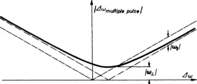
A. IDEAL WAHUHA AND MREV CYCLES 95 tells us that the suppression of dipolar interactions starts to become effective as soon as τ—not tc—becomes shorter than T2rigid. In view of the results of the early solid-echo experiments^84-87 this is but natural—in retrospect.

An interesting point to note is that ^^{2 )} vanishes for so-called two-spin systems.⁸⁸ Otherwise stated, ^^{2 )} contains no terms proportional to (l/rfk)³ but only terms proportional to (l/rffc)²(l/rfi), ΙΦ k, etc. In substances with pairs of closely neighbored protons, e.g., methylene groups or water mole- cules, the pair interatomic distance rik is considerably smaller than all other interatomic distances. The absence of terms (\/rfk)³ in ^^{2 )} means that the potentially largest terms, as far as geometry is concerned, actually do not contribute to if^²⁾ and, hence, to the broadening of the spectral lines.

The offset second-order correction term is

* £ > = -Δω(Δα>ν/18){(/χ+/,+/ζ) + 3 ( /ζ- / , ) } . (5-2) The rotation imposed on the spins by the (Ix + Iy + Iz) part is along the same

axis as results from the zeroth-order term. It therefore modifies—slightly—

the scaling factor. Instead of 1/^/3 it now becomes (l/x/3)(l— Δω²τ²/6).

As the sampling rate in a WAHUHA experiment is \/tc the maximum frequency (Nyquist frequency vN) in the spectrum is vN = \/2tc = 1/12τ.

The frequency-dependent correction to the scaling factor therefore never exceeds 4π²·3/6·12² = 0.138 = 13.8%. (The factor 3 enters because the spectral frequencies are scaled frequencies, whereas Δω is the unsealed off- resonance frequency.) Our experiments are usually arranged so that the highest frequency of interest in the spectrum is below £vN, where the cor- rection is about 3.5%. In our work on protons we even remain below £vN— there the correction is negligible.

The rotation of the spins due to the (I2 — Ix) part in Eq. (5-2) is perpendicular to the main rotation. It therefore affects the scaling factor only in second order.

However, it also tilts the rotation axis away from the rotating frame 111 axis.

The maximum tilt angle is 18.5°, which applies for the Nyquist frequency.

It is a matter of course that everything we have said about the offset second- order correction term applies equally well to the chemical shift second-order correction term.

Cross terms. It is clear that there is a multitude of cross terms involving

^cs> ^off> «*D> ^{a n}d «#j. The cross term quadratic in 3^Ώ and linear in Jfoff—

8 41. G. Powles and P. Mansfield, Phys. Lett. 2, 58 (1962).

8 51. G. Powles and I. H. Strange, Proc. Phys. Soc, London 82, 6 (1963).

86 R. Hausser and G. Siegle, Phys. Lett, 19, 356 (1965).

87 G. Siegle, Z. Naturforsch. A 21,1722 (1966).

88 B. Bowman, M.S. Thesis, Massachusetts Institute of Technology, Cambridge, 1969 (unpulished).

presumedly the most important one—is given by

(τ² Δω/18){2[JfD*, [JTD», / J ] + 2 |>rD«, [JTD», / J ]

- [jfD*. [JfD*,/J] + [/„[JTD*, JfD*]]}. (5-3) The damping constant associated with this term is proportional to

T (T2, rigid _ J _ \

Y 2'^{r i g i d}^ τ ' τ Δ ω /

Note that the damping increases linearly with the offset! We avoid writing expressions for other cross terms because they can be expected not to limit the resolution in actual experiments.

2. MREV EIGHT-PULSE CYCLE

This cycle was first described by Mansfield⁸³ as one of an entire family of eight-pulse, 12τ complementary cycles that compensate for both finite pulse width and rf inhomogeneity effects. Rhim et al.⁶⁷ first used it in 1973 in actual experiments and got amazingly good line-narrowing results. Later it turned out, however, that the improvement resulted to a small extent only from the particular sequence and more so from an overall improvement of the apparatus.

We describe here the properties of the ideal MREV eight-pulse cycle insofar as they differ from those of the WAHUHA cycle.

a. Properties Related to the Detection of the NMR Signal

The initial amplitude of the oscillating part of the NMR signal can be made equal to the initial amplitude of a free-induction decay signal by applying a properly chosen 90° preparation pulse (see Fig. 5-1). The maximum potential signal amplitude can thus be exploited fully with ease. The oscillating signal does not ride on a dc pedestal as it does with the WAHUHA sequence. The absence of the pedestal is of particular importance when spin-lattice relaxa- tion and/or (weak) IS dipolar couplings cause in WAHUHA experiments a decay of the pedestal, which is considerably inconvenient for the subsequent processing of the data.

b. Properties of Zeroth-Order Average Hamiltonian

First-rank /-spin interactions are retained, but scaled down by a factor of V^/3, which is smaller than the corresponding WAHUHA scaling factor.

c. First-Order Corrections

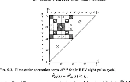
The total MREV eight-pulse cycle is not symmetric; hence, Jf⁽¹⁾ does not vanish identically. With the aid of Fig. 5-3 it is easily verified that the offset (Δω) and chemical shift (Δω,·) first-order correction terms are given by

■*&> + ^ = - * τ Σ (Δω + Δω,)²(Ij-lj). (5-4)

A. IDEAL WAHUHA AND MREV CYCLES 97

0 3T 6T 9T fc

FIG. 5-3. First-order correction term J^⁽¹⁾ for MREV eight-pulse cycle.

J?cs(0 + - ^ f f ( 0 ° C /e.

Domains φ and ® encompass symmetric subcycles and do not contribute to Jf⁽¹⁾. Domains 2χ - 24 are equivalent. <^02) and ^ ( / i ) commute in cross-hatched areas. Contributions from areas marked by crosses cancel.

The first-order dipolar correction term vanishes: Domains φ and ® in Fig.

5-3 encompass symmetric subcycles that do not contribute to if⁽¹⁾, and domain (2) involves the sum JfDx + J4?Dy + J^OZ = 0. The same arguments imply that the first-order dipolar-offset and dipolar-chemical-shift cross terms vanish.

d. Second-Order Corrections

The purely dipolar second-order correction term is identical with the corresponding WAHUHA term if it is written in terms of τ instead of tc. There are again cross terms between ^fD, J>fcs, ^foff, and JfJ. The coefficients are of the same order of magnitude as for the WAHUHA sequence.

From this enumeration the following conclusions may be drawn:

(i) The ideal (later) MREV cycle is hardly superior to the ideal (earlier) WAHUHA cycle. In Section D, where we consider pulse imperfections, it will become obvious that the MREV cycle is superior to the WAHUHA cycle.

(ii) The resolution "should" be best close to resonance since the second- order cross terms between JfO and J«foff vanish at, and are very small close to resonance.

(iii) <#£²⁾ appears to be the resolution-limiting factor.

Experimentally it is found in agreement with (ii) that the resolution deteriorates far off resonance^89,90; however, since our early multiple-pulse experiments

89 W. K. Rhim, D. D. Elleman, and R. W. Vaughan, /. Chem. Phys. 59, 3740 (1973).

90 A. N. Garroway, P. Mansfield, and D. C. Stalker, Phys. Rev. B 11, 121 (1975).

on CaF24 6 , 5 1 it became clear that the resolution tends consistently to be better somewhere off, rather than exactly on resonance. Later we realized that this is due to a further averaging process, which becomes operative off resonance and which we are going to describe now.

B. Off-Resonance Averaging

We start by recalling that the suppression of homonuclear dipolar couplings discussed so far is the combined result of two averaging processes:

(i) The application of a strong magnetic field Bst imposes a fast common motion on the spins, which makes it possible—even mandatory—to truncate the full dipolar Hamiltonian. We are left with the truncated or secular dipolar Hamiltonian, which is just the time average of the time-dependent full dipolar Hamiltonian in the rotating frame. There was and is no need at this stage to consider corrections ÜF⁽¹⁾, «#⁽²⁾, etc., to the average Hamiltonian because the Larmor period—which plays the role of the cycle time—is typically smaller by three orders of magnitude than T2 rigid in very low, in principle in zero, applied field.

(ii) The application of any one of the line-narrowing multiple-pulse sequences swirls all spins synchronously around and leads to a zero average of the truncated dipolar couplings in the toggling frame. Because the cycle time of the multiple-pulse sequence typically cannot be made much smaller than T2 rigid in high fields we had to consider correction terms to the average Hamiltonian. The lowest order nonvanishing purely dipolar correction term is ^²> for both the WAHUHA and MREV cycles.

The effective Hamiltonian in the toggling frame with the applied field set somewhat off resonance consists of

(i) a zeroth-order resonance-offset term, the detailed structure of which depends on the particular pulse sequence at hand,

(iii) a host of cross terms,

(iv) a host of pulse imperfection terms.

All these terms have equal rights in the effective Hamiltonian irrespective of whether they arise just as averages or as higher order correction terms.

In the toggling frame the resonance-offset term imposes a common uniform motion on all spins of a given isotopic species. It is just a third repetition of our by now familiar game to treat this common motion of the spins by a further interaction representation, Uoff. The consequence is that the remaining parts

B. OFF-RESONANCE AVERAGING 99 of the toggling-frame effective Hamiltonian—^^{2 )}, cross terms, pulse im- perfection terms—acquire a time dependence, e.g.,

Over this time dependence we may average eventually—provided it is fast enough.

Uof{ represents a rotation

(i) about the toggling-frame 111 direction for the WAHUHA four-pulse sequence,

(ii) about the toggling-frame 101 direction for the MREV eight-pulse sequence.

It is over these motions that we must average the time-dependent toggling- frame Hamiltonian. (Recall that the toggling and rotating frames can be considered to coincide if the spin system is observed stroboscopically.)

What is the result of this third averaging process? First of all, the time average of UF^²⁾(0 vanishes for the WAHUHA four-pulse experiment! It is possible, but rather tedious, to demonstrate this for a continuous rotation about the 111 toggling-frame axis (see Appendix C). It is much easier—and still sufficiently instructive—to consider a stepwise rotation with three steps for one full turn. This we shall do now.

We expressed iF£²⁾ in terms of ^Dx, jTOy, and JfDz. The structure of 3tfDx

etc., is evidently such that each 120° rotational step about the 111 axis carries successively

x -> y, y -> z, z -> x.

The averge of J ^^{2 )}( 0 becomes

+ [(XJ-X&IXJ,*^}. (5-5) A consequence of 3Vax+3VOy+3tfOz = 0 is

The inner commutators in Eq. (5-5) can therefore be bracketed out and the terms of the remaining factor cancel. Hence we have the result that the average of Jp£²⁾(0 vanishes for the WAHUHA sequence.

Off-resonance averaging substantially reduces but does not eliminate completely JF£^{2 )} for the MREV eight-pulse sequence. The direction of the off-resonance rotation axis is not as favorable as for the four-pulse sequence.

Let us ask now: How important is off-resonance averaging in practice?

This question is, in fact, somewhat too general. Therefore, let us ask in more detail:

(i) What about experiments that clearly demonstrate the effectiveness of off-resonance averaging?

(ii) What consequence has off-resonance averaging for the design of highly efficient line-narrowing multiple-pulse sequences?

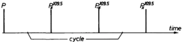
(i) Simple, rather than sophisticated, multiple-pulse sequences are best suited for demonstrating the effectiveness of off-resonance averaging. An example is the phase alternated tetrahedral angle (PAT) sequence⁹¹'⁹² sketched in Fig. 5-4.

On resonance, the PAT sequence does not average out the dipolar couplings between / spins. In fact, no pulse sequence consisting of two rf pulses only can do that.⁵¹ Indeed, in an experiment on resonance on CaF2, we could lengthen the decay of the ¹⁹F NMR signal barely by a factor of two.

Off-resonance averaging theory predicts a complete suppression of the /-spin dipolar couplings,⁹¹ and indeed a more than threefold stretching of the decay—as compared with the on-resonance case—was observed on going off resonance by 8 kHz.⁹¹

Pines and Waugh⁹³ realized that the stretching of the decay in this particular experiment was limited by a finite pulse-width effect, and that it could be overcome by adapting the nutation angle to the duty factor 2/w/ic of the sequence. These authors report having attained with the PAT sequence a ¹⁹F decay time in CaF2 in excess of 1 msec. They also give further examples of simple pulse sequences with marked off-resonance averaging effects together with a very intricate theory.

(ii) While there is no doubt that off-resonance averaging helps improve resolution with WAHUHA four- and MREV eight-pulse sequences there is

p/09.5 pH)9.5 pKJ9.5

time

T

zr

FIG. 5-4. The phase alternated tetrahedral angle (PAT) sequence. P is a preparation pulse and may be just another PI⁰*⁵ pulse.

9 1 U. Haeberlen, J. D. Ellett, and J. S. Waugh, / . Chem. Phys. 55, 53 (1971).

9 2 J. D. Ellett, Ph.D. Thesis, Massachusetts Institute of Technology, Cambridge, 1970 (unpublished).

9 3 A. Pines and J. S. Waugh, / . Magn. Resonance 8, 354 (1972).

C. T|| AND T±; HETERONUCLEAR DIPOLAR COUPLINGS 101

doubt that for the four-pulse sequence the improvement results predominantly from the suppression of «#^²⁾. We are led to this suspicion by the fact that the MREV eight-pulse sequence—where iF£²⁾ is not fully eliminated by off- resonance averaging—seems to yield significantly better resolution than the four-pulse sequence, where ^ ^{2 )} is fully eliminated.

A side conclusion from this observation is that there is no practical point now to use sophisticated multiple-pulse sequences for which not only ifD = jpv-) = 0, but also JF^²⁾ = 0. The first such sequence has been proposed by Evans,⁹⁴ and Mansfield⁸³ has devised a whole family of sequences that possess this property.

So, what gets eliminated by off-resonance averaging in WAHUHA and, above all, in MREV experiments? We get a hint by noting that the amount by which the field has to be set off resonance in order to attain the best resolution tends to become smaller and smaller as experimenters improve their equip- ment more and more. This indicates that off-resonance averaging is also effective in suppressing adverse pulse imperfection effects. With "poor"

equipment this is probably the most important off-resonance effect in MREV and WAHUHA experiments.

We shall study pulse imperfections rather carefully in Section D, but first we shall consider another interesting resonance offset property of multiple- pulse sequences, namely, a dramatic difference in relaxation rates parallel and perpendicular to the effective field in the toggling frame.

C. T|| and Γ±; Heteronuclear Dipolar Couplings

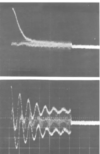
Consider Fig. 5-5, which is taken from Haeberlen et al.⁹¹ It shows the

1 9F NMR signal of CaF2 in an on- and an off-resonance WAHUHA experiment.

On resonance, the magnetization <M> decays nearly to zero over the time of the WAHUHA experiment, off resonance it does not. The oscillations almost do, but not the pedestals. As we have seen in Chapter IV, the pedestals arise from the component of <M> that is initially parallel to Beff in the toggling frame, whereas the oscillations arise from the component of <M> that is perpendicular to Beff. For convenience we shall characterize by time constants T± and T|| the decays of <M>, respectively, perpendicular and parallel to Beff, even though these decays need not be simple exponential. TL corresponds to the usual WAHUHA decay time. That two relaxation rates are involved in NMR line-narrowing experiments had already become evident from the work

W. A. B. Evans, private communication (see Haeberlen and Waugh⁵¹)·

FIG. 5-5. WAHUHA experiment performed on a single crystal of CaF2. Horizontal scales = 1.0 msec/division. Upper trace, on resonance; lower trace, 2.0 kHz off resonance (from Haeberlen et al.⁹¹).

of Lee and Goldburg⁶¹ and Tse and Hartmann.⁹⁵ In both of their experiments solid samples were irradiated with a strong rf field whose intensity and frequency offset from resonance were chosen to produce an effective field in the rotating coordinate frame, which made the magic angle with the z axis.

Lee and Goldburg measured the rate of decay (Τ±_1) of the component of

<M> perpendicular to the effective field, while Tse and Hartmann studied the relaxation (T^) of the magnetization along Beff and they found Γ|( to be orders of magnitude longer than TL as found by Lee and Goldburg.

95 D. Tse and S. R. Hartmann, Phys. Rev. Lett. 21, 511 (1968).

C. Γ|| AND Τλ; HETERONUCLEAR DIPOLAR COUPLINGS 103

In one experiment we measured T{1 in an off-resonance WAHUHA experi- ment on a single crystal of CaF2 doped with paramagnetic U⁴⁺ ions and found it to exceed 0.6 sec, which is two orders of magnitude greater than its on- resonance value. (A Ty of 0.6 sec exceeds the spin-lattice relaxation time 7i of that crystal. This is possible because in the WAHUHA experiment, as in the experiment of Tse and Hartmann, the spin diffusion relaxation mechanism is suppressed.) T± only increased by a factor of roughly three on going the same amount off resonance.

We can use the resonance offset-averaging theory to understand in a qualitative way the difference between the resonance offset dependences of T|| and T±. The on-resonance decay of the magnetization is determined by iP^²⁾ and pulse imperfections. We have seen above that off resonance we must average these correction terms over the motion caused by Beff in the toggling frame. As in Chapter IV, Section C,4,d, it is again helpful to introduce a new set of axes in the toggling frame, the Z axis of which points along the (old) 111 direction. The average of a typical correction term if|ⁿ⁾ over the motion generated by Beff has the form

<^iP("^>>- = γπ j^expWV&ptxpi-MIz)**.

This expression commutes with 7Z, which we can easily see if we express JFj^ⁿ⁾ in terms of spherical tensor operators Tlm to take advantage of their simple transformation and commutation properties.

<c#A(n)>av can be written as a sum of terms of the form

Γ\χρ(ίΦΙζ)Τ1ηί exp(-/0/z) άΦ = — j \xp(imQ>)Tlm άΦ = Sm0Tl0. But[/z,Tz o] = 0.

Therefore, back in the old toggling frame (or rotating frame if observation of the spin system is restricted to the proper windows) we have

[ < ^ i^{M )}> a v , ( / x + / , + / z ) ] = 0 .

Thus, for a sufficiently large resonance offset the correction terms to the on-resonance average Hamiltonian are replaced by terms that commute with (Ix + Iy + Iz). It follows immediately from this and the equation of motion (Heisenberg equation) for the magnetization operator M ( 0 ,

tö(0 = '{(lI<^i'

>av+-),M(/)l,

that the time derivative of the component of the magnetization parallel to the 111 direction in the toggling frame is zero. [The dots indicate higher order

1

2K

corrections to the present averages.] This accounts for the fact that in multiple- pulse line-narrowing experiments performed off resonance the components of

<M> parallel to the 111 direction decay much more slowly than the com- ponents of <M> perpendicular to that direction.

On resonance, T± is determined by a number of correction terms, some of which commute with (Ix+Iy+Iz) and some of which do not. Off resonance, only terms that commute with (Ix + I_z + I_y) remain to first order, so that T±

increases somewhat off resonance, but not so much as Ty, which is not affected at all by these terms. Since the average chemical-shift Hamiltonian jfcs

commutes with (Ix + Iy + Iz), the Heisenberg equation of motion above implies that the component of <M> along the 111 direction will not carry information about the chemical shifts of the sample. Thus we see that Tl9 rather than Τ|(, gives a measure of the chemical shift resolution of a multiple-pulse line- narrowing experiment.

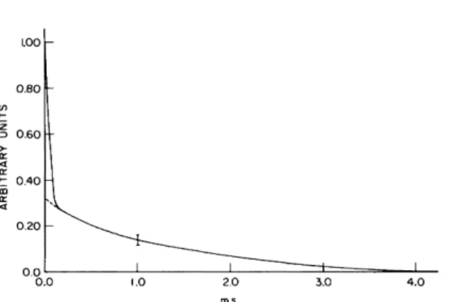
In crystals containing more than one species of nuclear spins the WAHUHA T|| is much greater than TL both on and off resonance. Figure 5-6 (again from Haeberlen et al.⁹ⁱ) shows the WAHUHA ¹⁹F decay of a single crystal of LaF2. Notice that there is a rapid initial decay of the signal train to « ^ of its initial value, followed by a much slower decay. The initial decay time is 48 //sec, which is longer than the 20.2 /zsec ¹⁹F free-induction decay time of the crystal at this orientation. The slowly decaying signal never develops a beat structure as the spectrometer frequency is shifted away from resonance, although the time constant of the decay decreases as the resonance offset is increased beyond several kilohertz. The difference between T^ and T± in this experiment follows from the nature of the truncated heteronuclear dipolar interaction Hamiltonian, ^s^ifar, which in this experiment dominated the decay.⁹⁶ It behaves in the /-spin space as a first-rank tensor so its average during the pulse sequence, both on and off resonance is

« f , r = iy

y

l>T

V-3cos

!)

)s

(i

+i

+i

).

i,k

As usual, the /-spin species (¹⁹F) is the one we observe and hit by the multiple- pulse sequence. This average Hamiltonian commutes with (Ix + Iy + Iz) and as noted earlier, this implies that the decay of the component of <M> along the 111 direction will be slower than the decay of the component of <M>

perpendicular to that direction. Thus T^ should exceed Tl9 as indeed is the case in Fig. 5-6. The resonance offset average Hamiltonian commutes with (Ix + Iy + Iz), which accounts for the fact that no beat structure was observed on the slowly decaying signal.

96 Suppression of ^RciL· by either heteronuclear or self-decoupling has been discussed in Chapter IV, Section F,5.

D. PULSE IMPERFECTIONS 105

1.00

0.80

§ 0.60

<

t 0.40

CD <

0.20

"'O.O 1.0 2.0 3.0 4.0 ms

FIG. 5-6. WAHUHA experiment performed on a single crystal of LaF2 (from Haeberlen etal⁹¹).

D. Pulse Imperfections

Naturally we can never excite our spin systems with ideal pulses in real experiments. Since the averaging achievable with ideal pulse sequences—

which we have considered thus far—appears to be fantastically good, and since the results of the pioneering experiments in all multiple-pulse laboratories were or are not that good, suspicion has arisen that the discrepancy is due to pulse imperfections. We are aware of a host of pulse imperfections and there may be more we are not aware of. For most of the pulse imperfections that we understand, compensation schemes have been worked out. We shall discuss them in this section.

The following pulse imperfections have attracted interest thus far:

finite pulse widths,

flip angle errors common to all pulses, rf inhomogeneity,

power droop,

flip angle errors different for the different sets of pulses, phase errors,

phase transients.

We shall consider here another conceivable imperfection, namely, timing errors.

1. FINITE PULSE WIDTHS; COMMON FLIP ANGLE ERRORS;

rf INHOMOGENEITY; POWER DROOP

These pulse imperfections form a class to which we shall turn first. Their important common feature is that they do not destroy the cyclic and the

symmetry properties of multiple-pulse sequences (see below). For a power droop this is true only in so far as the power droop over individual cycles can be neglected. Our approach will be completely straightforward: We consider the average Hamiltonian of spin systems subject to multiple-pulse sequences composed of pulses of finite width that flip the nuclear magnetization through variable angles ß. We shall learn how the zeroth-order effects of finite pulse widths can be overcome.⁹⁷ We shall further learn to understand the sensitivity of various pulse sequences to flip angle errors common to all pulses and thus also to a droop of the rf power in the course of a long pulse train. Our approach also provides an understanding for the effects of rf inhomogeneity since rf inhomogeneity means nothing but a distribution over the sample volume of common flip angle errors. Again we shall start by considering the WAHUHA cycle. The (superior) properties of the MREV eight-pulse cycle can easily be inferred from those of the WAHUHA four-pulse cycle.

As this class of pulse errors does not destroy the symmetry properties of multiple-pulse sequences, the WAHUHA sequence remains symmetric even when the pulses have a finite width. As a result all corrections of odd order to the average Hamiltonian still vanish automatically (see Chapter IV, Section D,4). We think it is reasonable to suspect that second-order corrections, and higher order corrections of even order in general, are modified only slightly by pulse imperfections—which we are trying to keep down anyhow—so it is not worthwhile going through the trouble of studying them for imperfect pulse cycles.

a. WAHUHA Four-Pulse Cycle with Pulses of Finite Width;

Condition for JfD = 0; Scaling Factor

Figure 4-2 shows the timing of a WAHUHA sequence with pulses of finite width. Also shown is the evolution of the propagation operator UTf(t), which is evidently symmetric about the midpoint of the second large window. The last two columns of Fig. 4-2 are intended to provide a "look and see" proof of that fact. Since Urf(t) is symmetric, J4?j^nt(t)= U~{ 1 (t)^sl^ulaT UT{(t) is also symmetric. The consequence of this property of ^^nt(t) with regard to JF⁽¹⁾ has been mentioned above. Another consequence is that for evaluating i f it is sufficient to consider only one half of the cycle. The average of -ocular (0> ^m particular, is proportional to

1 ^

r. i* - 3</

(o/

(/)>

= r. i* - - 2 3</;(0//(0V

p=l

where the summation is over the intervals p = 1,..., 5 of the first half of the WAHUHA cycle; <···>ρ means average over interval p\ tpis the duration of interval p.

M. Mehring, Z. Naturforsch. A 27, 1634 (1972).

TABLE 5-1 AVERAGES OF Ij(/)//(/) OVER INTERVALS /?= 1,...,5 OF WAHUHA SEQUENCE (SEE FIG. 4-2)a Coefficient of 5 τ

/,'/** W h%k i(h%k + VA*) i(h%k + W) «/,'/,* + /,'/,*)

~ : ^ : : r -

It is straightforward to evaluate the averages (Ιζ((ί)ΙζΗ(ί)}ρ. The heading in Table 5-1 shows which operator forms are generated by UTf (t) from IZIZ. The further entries of the table show the coefficients, multiplied by tp, of these operators in the averages (Iz((t)Izk(t)yp.

The average of ^s«uiar(0 contains, of course, the same spin operator combinations as does the heading in Table 5-1. The coefficients of these operators in the average of «^c uia r(0 are given in Table 5-2. Starting from Table 5-1, only simple juggling with trigonometric functions is required to find the expressions of Table 5-2.

The outstanding feature of Table 5-2 is that all the coefficients have one factor in common. Suppression of dipolar interactions is evidently obtained when this factor becomes zero, which means when

In Eq. (5-6) let us consider ίψ/2τ as a parameter and the flip angle β = ωίίγ/

as a variable. Note that this assignment of roles follows closely at least a possible procedure of alignment of actual multiple-pulse sequences. The range of ίψ/τ is clearly 0 ^ rw/ r ^ l . The equality signs apply only for idealized cases. By a different approach, which did not state the problem as clearly as do Table 5-2 and Eq. (5-6), we recognized very early⁵¹ that ^s?c u l a r

can be suppressed not only for iw = 0, but also for small but finite values of the parameter fw/r. However, it was Mehring⁹⁷ who realized—still using a somewhat different approach—that there is a choice of β for the entire range of

TABLE 5-2

AVERAGE OF Γ · Ι * - 3 /Ζ7Ζ* OVER W A H U H A FOUR-PULSE CYCLE WITH PULSES OF FINITE WIDTH /wa

Operator Coefficient

IJU

Ι,Ί," [ - ] COS³£

/Z7Z* - [ . . ] ( l + cos²)9)cos^

Wx%^k + h%^k) - [ - ] 2sin²£ HW+UIS) -[···] 2 sin 2ß i(/„7x*+/,7/) -[...](l + cos²£)2sin)ff

a The coefficients of the relevant spin operator combina- tions in <I'-I*—3/z7zk>av are shown. The expression in the square brackets, [···], is the same in all coefficients.

D. PULSE IMPERFECTIONS 109 tyf/τ that satisfies Eq. (5-6). We shall denote the particular value of the flip angle ß that satisfies Eq. (5-6) by ß0, which is a function of *W/T.

For tyf/τ = 0, ß0 is, of course, equal to \π. For ίψ/τ = 1, Eq. (5-6) leads to the transcendental equation tan/?0 = — β0, which has β0 — 116.24° as a solution. For intermediate values of JW/T, β0 varies monotonically between these two limiting values. Mehring⁹⁷ gives a plot of β0 versus f/w/r (which is the duty factor of the pulse train).

In our experiments we usually select a certain value for *W/T, typically 0.2.

Then we adjust β for optimum resolution. If everything is aligned properly we indeed obtain the optimum resolution for β slightly larger than \π.

In summary, homonuclear dipolar interactions can be suppressed up to and including first-order corrections in the Magnus expansion by WAHUHA four-pulse sequences with pulses of finite width. The condition is that the flip angle β is chosen such that it satisfies Eq. (5-6) for the selected ratio of fw/τ.

Finite pulse widths affect not only the suppression of dipolar interactions, but also the scaling factor and, weakly, the off-resonance averaging mech- anism. To study their influence on the scaling factor we must consider the average of Iz(t). This is easily obtained with the aid of Fig. 4-2. We give only the result:

</,(0>.v

= <^I7¹(0/,t/r f(0>.v

1 Ι * Γ · R 'w/sinj? 1-cosjgyi

+ /, (l+cosj3+cos²)3)

tv/f _ l + c o s²ß /t 0^^sinß

cosj5 + ^—£ - (1 +cosj?) —f (5-7)

Denoting the coefficients of Ix, Iy, and Iz in Eq. (5-7) by Cx, Cy9 and Cz, respectively, the scaling factor S may be expressed by

S = KCX2 + Cy2 + Cz2)¹¹². (5-8)

With the aid of any decent pocket-sized calculator it is easy to verify that S varies monotonically between 3 "^{1 / 2} = 0.57735 and 0.56606 as fw/r increases from 0 to 1, provided β is always chosen such that it satisfies Eq. (5-6). This very small variation of the scaling factor S is of no practical importance,

particularly as S is an easily measurable quantity. We are, of course, very glad that in return for being able to work with increased pulse widths we do not have to pay a high price in terms of an appreciably reduced scaling factor.

b. Flip Angle Errors Common to All Pulses; rf Inhomogeneity;

Power Droop

State-of-the-art multiple-pulse spectrometers usually have a means to monitor the pulse power of the transmitter. By turning on the corresponding knob one adjusts for the optimum flip angle ß0. Misadjustments lead to flip angle errors common to all pulses. Much more dangerous are, however, flip angle errors that are not under control of the spectroscopist. (We contrast the spectroscopist to the designer and builder of the spectrometer although often they are the same person.) Such errors are caused by, e.g., all short- and long-term variations and drifts of the transmitter power output. The notorious power droop—the decrease of the transmitter power output during the course of a long pulse train—is just a special case. One source of these troubles is drifting and humming of dc power supplies. Another important source of common flip angle errors is the unavoidable rf inhomogeneity, which makes it impossible to adjust ß to its optimum value ß0 for all volume elements of the sample.

The discussion of common flip angle errors, rf inhomogeneity, and power droop is contained in a discussion of the dependence on ß of the NMR response of a solid sample to the particular multiple-pulse sequence at hand.

We shall study this dependence here for the WAHUHA sequence. Our main concern is, of course, spectral resolution. There are two main reasons why a deviation ε of β from its optimum value β0 (by definition, ε = β — β0) affects the resolution attainable in multiple-pulse experiments:

(i) ε φ 0 leads to an incomplete suppression of dipolar interactions.

(ii) ε Φ 0 changes the scaling factor 5, and this leads via the rf inhomo- geneity to a deterioration of the spectral resolution.

There is also an indirect consequence of flip angle errors: The variation with β of the direction of Beff in the toggling frame makes the resonance offset- averaging mechanism dependent on β. We only mention this effect but do not dwell upon it.

We are well prepared for our current subject: The dependence on ε of ifD = <«^s£ular(0>av i^s contained in the coefficients of Table 5-2, and the dependence on β of the scaling factor or, even more important, of

<7z(0>av ^ <^cs + ^)ff i^s contained in Eq. (5-7). For better perception of the sensitivity to ε of J-fD, ^ cS + ^ff > ^{a n}d the scaling factor, we have compiled in Table 5-3 the coefficients of the spin operator combinations occurring in JfD

and ^cs + ^>ff *ⁿ terms of ε for ίψ/τ -> 0.

D. PULSE IMPERFECTIONS 111

TABLE 5-3

SENSITIVITY TO e OF THE COEFFICIENTS OF THE SPIN OPERATORS OCCURRING IN <#D AND ^s+ « C f f^a

Operator

/,'/**

w

Uh^k [/,'/.']+

[/*'//]+

[ W ] +

', 4 h

Coefficient in J^D or sin²e

sin⁴e

— sin²e(l + sin²e)

— 4 cose sin²e 2 cos²e sine 2(1 + sin²e) sine cose cose

cos e(l —sine) 1 — sine + sin²e

JlQS ■+- ^0f f

-> e²

-►

-> - e² -> - 4 e² - > 2 e

-►2e -» 1 - e²/2

for ίψ/τ -*· 0 + 0(e⁴)

0(e⁴) + 0(e⁴) + 0 ( e⁴) + ö(e²) + 0(e³) + 0(e⁴) -► l - ( e + i e²) + 0(e³) -> l - ( e - e²) + 0(e³)

a [7p7g*]+ is an abbreviation for ± ( W + /e'/p*).

The coefficients of [/*'//] + , [/^Λ^ + , /y, and 7Z depend linearly on ε. It is via the corresponding terms in J^D and Jfcs + <#off that the inhomogeneity of the rf field, a power droop, and a misalignment of the transmitter power affect by far most strongly the spectral resolution in WAHUHA experiments.

Residual dipolar line broadening is expressed by the first two of these terms, whereas the latter two lead—among other things—to line broadening via the rf inhomogeneity. In the following subsection we shall see that by combining variants of the WAHUHA sequence it is possible to eliminate all coefficients of bilinear spin operators that are linear in Iy. These are (what luck!) exactly those coefficients that are linear in ε and that are, as a result, the most disturbing. Therefore, we shall not discuss residual dipolar line broadening any further for the WAHUHA sequence.

On the other hand, it seems impossible to eliminate by this technique the coefficients linear in ε of linear spin operators, and thus the strongest direct line-broadening effect arising from rf inhomogeneity.

Garroway et al.⁹⁰ have shown, however, that by combining WAHUHA- type cycles with cycles that contain 270° pulses in addition to 90° pulses it is possible also to eliminate these terms. While the scheme has been proven to work well for liquids it remains to be seen whether it is also useful for solids.

The direct rf inhomogeneity line-broadening mechanism in WAHUHA experiments works as follows: In an rf coil there always exists a distribution of the strength Bx of the rf field, and consequently a distribution of ß over the sample volume. Let us assume that this latter distribution is centered at ß0, that it is bell-shaped, and that its half-width at half-height is <ε²>^1/2. Con- sider a narrow resonance line of a liquid sample, which in the ordinary NMR spectrum is shifted off resonance by Δω. The center of the line appears in the

multiple-pulse spectrum at AcoS(ß0). Spins that are flipped by angles ß different from ß0 "appear" in the multiple-pulse spectrum at AcoS(ß). S(ß) is given by Eq. (5-8). By expressing S in terms of ε and assuming for simplicity ίψ/τ <ζ 1, which means β0 « %π, we obtain

AcoS(ß) -> AcoS(ß0 + e) = Δω5(*π)(1+£β) = Aco(l/V3)(l.+ $e). (5-9) The distribution of the strength of the rf field is thus reflected directly in the multiple-pulse lineshape of a liquid sample. The half-width at half-height of the line is Aco(l/>/3)f <ε²>^1/2. Note, in particular, that the width increases linearly with the offset Δω. For WAHUHA experiments on liquids this is typically the dominant line-broadening effect. For solids it is one line- broadening mechanism among several others.

In order to get an idea of its practical importance let us choose <ε²>^1/2 = 0.052 ^= 3° and Δω = 2π x 2000 sec^{- 1}. These values lead to a line with a full width at half-height of as much as 2π χ 80 Hz. Both input numbers of our example are absolutely realistic: It requires special techniques and efforts to wind small rf coils that produce rf fields substantially more homogeneous over reasonably sized samples than specified by <ε²>^1/2 = 3°, although values less than 1° have been reported.⁸⁹ Δω = 2π χ 2000 Hz is a natural value to choose for the center of proton spectra, which at ω0 = 2π χ 90 MHz have a typical spread of 2πχ2250 Hz = 25 ppm. For ^{1 9}F work even substantially larger off-resonance shifts are often required.

c. Residual Dipolar Line Broadening; Compensation Schemes;

MREV Eight-Pulse Sequence

With regard to residual dipolar line broadening, we recognized those terms in Tables 5-2 and 5-3 as the most dangerous ones that are linear in ε. As we have shown in 1968⁵¹ it is possible to design compensation schemes that eliminate these troubling terms. The most successful of them—up to this date—seems to be the MREV eight-pulse sequence (see Fig. 5-1), which consists of two subcycles: the first is a WAHUHA cycle; the second is again a WAHUHA cycle, but the Px and P_x pulses are interchanged. The propa- gation operator Ur{(t) runs during the first MREV subcycle through exactly the same sequence of states as it does in a WAHUHA sequence. During the second subcycle Urf (t) runs again through the same sequence of states, but the sign of Ix is reversed everywhere.

Let us consider «?fD for the MREV sequence. The spin operator combinations involved are the same as for the WAHUHA sequence (see Table 5-2). The coefficients are one-half the sum of the respective coefficients from each sub- cycle. For the first one they are evidently identical with the corresponding coefficients of the WAHUHA cycle (see Table 5-2). We leave it as an easy exercise for the reader to show that the same coefficients are obtained again

D. PULSE IMPERFECTIONS 113 for the second subcycle; however, the signs are reversed of all those coefficients belonging to operators that contain Iy linearly.

As a result, the MREV-coefficients of [Ix%^kli + and Uy%^k1 + vanish identi- cally, that is, regardless of the particular value of ß. A corresponding result is obtained for J^cs and Jfofi: The coefficient of Iy vanishes identically.

These results have highly important consequences: All remaining co- efficients in 3tfO now have two factors in common, namely,

( ⁱ " ?) ^cosjS+ ? \ ^sin H ^{and cosj8} *

This means that there are now two possible choices of β for which ifD vanishes.

One is the same as for the WAHUHA cycle [see Eq. (5-6)] and the other is β = \π. Both choices coincide for ίψ/τ = 0.

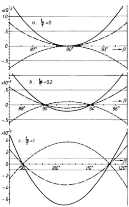
Figure 5-7 shows how the surviving coefficients in «?fD vary with β for three choices of *W/T. The interesting point to note is that they all stay very small—

below 1%, say—for an appreciable range of β. This is true, in particular, when ίψ/τ is, on the one hand, nonzero so that the two zeros of JPO are well separated, but when, on the other hand, it is small enough for the coefficients to remain negligibly small between the zeros. Figure 5-7c shows that this is definitely no longer the case for large pulse widths approaching the limiting case fw -» τ. It is therefore not advisable to operate MREV sequences with pulse widths approaching τ.

In summary, we may say that for small (but nonzero) pulse widths the sup- pression of dipolar spin-spin couplings by the MREV eight-pulse sequence is very insensitive to flip angle errors common to all pulses and therefore to misalignments, fluctuations, drifts, and a droop of the rf pulse power, and to the inhomogeneity of the rf field.

These properties of the MREV eight-pulse cycle—first predicted theoret- ically by Mansfield⁸³—have been confirmed by specific experiments⁵⁵ and are confirmed by daily work in multiple-pulse laboratories—including ours—

all over the world.

What about the direct rf inhomogeneity line-broadening mechanism in MREV experiments? For the WAHUHA sequence the coefficients in JPCS

and Jfof{ of both Iy and Iz are linear in ε. Only the coefficient of Iy is thrown out with the MREV sequence, so that we are left with one coefficient linear in ε.

The counterpart of Eq. (5-9) is for the MREV sequence

foriw/T->0

AcoS(ß) - AcoS(ß0 + e) = ΔωΑ(*π)(1 +$e) = Δω^V2(l +$e).

(5-10) By comparing Eqs. (5-9) and (5-10) we see that the direct rf inhomogeneity line-broadening mechanism is almost as effective for the MREV as for the

FIG. 5-7. Average dipolar Hamiltonian *^D for MREV sequence versus flip angle ß. The curves show the coefficients of iUx%^k + h%^K), ; /*'/**, ; and 7z72k, - - ; for three different choices of /_W/T. The coefficient of /,'//, though nonzero for βφ\π and /?₀, is always negligibly small. Note that the horizontal and vertical scales, respectively, are equal for /W/T = 0 and 0.2, but much larger for ίγ,/τ = 1. Note in particular the range of β for which all coefficients stay smaller than, e.g., 10" ². For /W/T = 0.2 this range exceeds 9°.

WAHUHA sequence. Carefully optimizing the homogeneity of the rf field is therefore mandatory if one wishes to exploit fully the capability of suppressing dipolar spin-spin interactions in solids with any of these multiple-pulse sequences.

2. FLIP ANGLE AND PHASE ERRORS OF INDIVIDUAL PULSES;

PHASE TRANSIENTS

We shall discuss this class of pulse imperfections together. Their common characteristic feature is that they destroy the cyclic property of multiple-pulse sequences. This means the propagation operator Urf(t) does not return to unity after a full cycle in the presence of these imperfections. While this seems