Comparison of analytical and numerical ground-state approaches

(1)

Editors’ Suggestion

Symmetric single-impurity Kondo model on a tight-binding chain:

Comparison of analytical and numerical ground-state approaches

Gergely Barcza,¹Kevin Bauerbach ,²Fabian Eickhoff,³Frithjof B. Anders ,³Florian Gebhard ,^2,*and Örs Legeza¹

1Strongly Correlated Systems Lendület Research Group, Institute for Solid State Physics and Optics, MTA Wigner Research Centre for Physics, P.O. Box 49, H-1525 Budapest, Hungary

2Fachbereich Physik, Philipps-Universität Marburg, D-35032 Marburg, Germany

3Theoretische Physik 2, Technische Universität Dortmund, D-44221 Dortmund, Germany

(Received 19 November 2019; revised manuscript received 27 January 2020; accepted 27 January 2020;

published 24 February 2020)

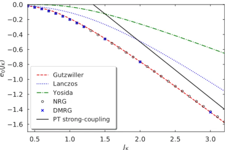
We analyze the ground-state energy, local spin correlation, impurity spin polarization, impurity-induced magnetization, and corresponding zero-field susceptibilities of the symmetric single-impurity Kondo model on a tight-binding chain with bandwidth W =2D where a spin-¹₂ impurity at the chain center interacts with coupling strength JK with the local spin of the bath electrons. We compare perturbative results and variational upper bounds from Yosida, Gutzwiller, and first-order Lanczos wave functions to the numerically exact extrapolations obtained from the density-matrix renormalization group (DMRG) method and from the numerical renormalization group (NRG) method performed with respect to the inverse system size and Wilson parameter, respectively. In contrast to the Lanczos and Yosida wave functions, the Gutzwiller variational approach becomes exact in the strong-coupling limitJKW, and reproduces the ground-state properties from DMRG and NRG for large couplingsJKW, with a high accuracy. For weak coupling, the Gutzwiller wave function describes a symmetry-broken state with an oriented local moment, in contrast to the exact solution.

We calculate the impurity spin polarization and its susceptibility in the presence of magnetic fields that are applied globally or only locally to the impurity spin. The Yosida wave function provides qualitatively correct results in the weak-coupling limit. In DMRG, chains with about 10³ sites are large enough to describe the susceptibilities down to JK/D≈0.6. For smaller Kondo couplings, only the NRG provides reliable results for a general host-electron density of states ρ0(). To compare with results from Bethe ansatz that become exact in the wide-band limit, we study the impurity-induced magnetization and zero-field susceptibility. For small Kondo couplings, the zero-field susceptibilities at zero temperature approach χ0(J_KD)/(gμB)²≈ exp[1/(ρ0(0)JK)]/[2CD√

πeρ0(0)JK], where ln(C) is the regularized first inverse moment of the density of states. Using NRG, we determine the universal subleading corrections up to second order inρ0(0)JK.

DOI:10.1103/PhysRevB.101.075132

I. INTRODUCTION A. Kondo problem and Kondo model

Magnetic moments that couple antiferromagnetically to electron spins of a metallic host pose a difficult many-particle problem because the spin-flip scattering of the host electrons off the impurity spin couples the bath degrees of freedom in an intricate way. Experimentally, this leads to surprising phenomena such as the Kondo resistance minimum around some characteristic low-temperature energy scaleTK[1], often referred to as the Kondo temperature.

Using standard high-temperature perturbation theory to third order in the coupling between the impurity spin and the host electrons, Kondo was able to explain the resistance minimum [2]. However, within standard perturbation theory the resistivity and many other physical quantities like the zero-field magnetic susceptibility diverge logarithmically at

*florian.gebhard@physik.uni-marburg.de

zero temperature. A summation of the leading logarithmically diverging terms in the perturbation expansion leads to a divergence at TK [3,4]. Consequently, approaches beyond perturbation theory are required to describe adequately the ground state of the coupled system of impurity spin and host electrons [4].

This “Kondo problem” inspired the development of scaling concepts that were eventually formalized in Wilson’s renormalization group (RG) [5]. Since the Wilson RG can be carried out analytically only to a limited degree, it found its widespread implementation as numerical renormalization group (NRG) method which is best suited for the study of impurity problems [5–7]; for a review, see Ref. [8].

At zero temperature, the impurity spin and the electrons in its surrounding “Kondo cloud” form a “Kondo singlet”

as the many-particle ground state; its elementary excitations describe a Fermi liquid [9]. The Bethe ansatz permits the exact solution of the Kondo model with infinite bandwidth (see the reviews by Tsvelick and Wiegmann [10] and by Andrei, Furuya, and Lowenstein [11]). The Bethe ansatz confirms the findings of (N)RG, and provides analytical formulas, e.g.,

(2)

for the impurity magnetization at finite temperatures, and for the Kondo temperature in terms of the Bethe-ansatz parameters. Since NRG provides explicit results also for dynamical quantities at finite temperatures, the Kondo problem could be declared “solved.”

The Kondo problem poses one of the fundamental chal- lenges in theoretical many-body physics. Therefore, one might think that the ground-state properties of the Kondo model have been studied in very much detail. Surprisingly, this is not the case. For example, the dependence of the ground-state energy on the Kondo coupling is largely un- known, apart from a study by Mancini and Mattis who used the Lanczos approach [12]. To the best of our knowledge, the large-coupling limit of the Kondo model has not been ana- lyzed extensively yet. Moreover, more elaborate variational states such as the Gutzwiller wave function were not applied to the Kondo model thus far.

It was not until recently that Schnack and Höck used the NRG to investigate the magnetization and zero-field susceptibility for some weak couplings [13]. They emphasized that the impurity spin polarization differs from the impurity-induced magnetization for the whole system, as derivable from the free energy. Moreover, they revived the question how the Bethe-ansatz results can be used for comparison with NRG data because the Kondo couplings in the Bethe ansatz and for a lattice model are related in a nontrivial way. For the series expansion of the Bethe-ansatz couplingJ_K^BA in terms of the bare model parameter JK, only the leading-order terms are known analytically from scaling arguments [4] and Wilson’s RG [5].

With our work, we fill some of the gaps in the quantitative analysis of the symmetric Kondo model at zero temperature.

We study the ground-state energy, the local spin correlation function, the impurity spin polarization and the impurity- induced magnetization as a function of a global and a local magnetic field, and the corresponding zero-field susceptibilities. In the absence of an external field, we perform weak- coupling and strong-coupling perturbation theory. We employ three analytical variational approaches (first-order Lanczos [12,14,15], Yosida [16,17], and Gutzwiller states [18,19]), and perform numerical calculations using the density-matrix renormalization group (DMRG) [20–22] and the numerical renormalization group methods [5–8,13]. We compare to Bethe-ansatz [10,11] results where possible.

B. Outline

Our work is organized as follows. In Sec.IIwe define the Kondo Hamiltonian on a chain and the ground-state properties that we investigate in the thermodynamic limit, namely, the ground-state energy, local spin correlation function, impurity spin polarization and impurity-induced magnetization, and the corresponding zero-field magnetic susceptibilities.

In Sec.IIIwe employ perturbation theory as first analytical method to derive the ground-state energy and the local spin correlation for weak and strong Kondo couplings. These results provide a benchmark test for all approximate analytical and numerical methods.

Next, in Sec. IV, we derive a variational bound for the ground-state energy from the first-order Lanczos state. As the

energy bound is poor, we refrain from calculating magnetic properties for this state.

As a more suitable variational state, we study the Yosida wave function in Sec.V. When properly generalized to finite magnetic fields, it permits the analytic calculation of magnetic ground-state properties in the presence of a local and a global magnetic field. Although the Yosida state gives a poor esti- mate for the ground-state energy, it provides a qualitatively correct description of the zero-field magnetic susceptibilities at small Kondo couplings.

As a third analytic variational approach, we study the Gutzwiller wave function in Sec. VI. It can be viewed as a Hartree-Fock ground state for the Kondo model where the condition of a spin on the impurity is guaranteed. From the Hartree-Fock perspective, it is not too surprising that the Gutzwiller state contains an artificial transition from a phase with a broken local symmetry at small Kondo couplings to a phase with a local spin singlet at large Kondo couplings. Apart from this flaw, the ground-state energy and the local spin correlation are in very good agreement with numerically exact data from NRG and DMRG. The Gutzwiller state becomes exact for strong couplings.

As the last analytic approach, we recall results from the Bethe ansatz in Sec. VII. The Bethe ansatz solves a related Kondo model that has a linear dispersion relation with an infinite bandwidth so that it is a nontrivial task to establish the link to the parameters in the lattice model. This is accomplished by Wilson’s renormalization group, and we use perturbation theory to calculate analytically the leading-order terms for the zero-field impurity-induced susceptibility.

In Sec.VIIIwe discuss two numerically exact approaches to the Kondo problem, namely, the numerical renormalization group (NRG) and the density-matrix renormalization group (DMRG) methods. The DMRG treats finite chains with up to L≈1000 sites with a very high numerical accuracy. Thereby, DMRG provides excellent variational upper bounds for the ground-state energy and the local spin correlation function.

Since it has an essentially constant energy resolution over the whole band, our present version of DMRG cannot access the exponentially small Kondo scale that develops for small Kondo couplings. The NRG was developed and designed to treat these Kondo scales and therefore provides access to small Kondo couplings as well.

In Sec. IX we compare the results of all methods. The Gutzwiller approach provides the best analytic variational state for the ground-state energy and the local spin correlation function. The Gutzwiller wave function becomes the exact ground state for large Kondo couplings, and reliably describes the physics when the Kondo coupling becomes larger than the host-electron bandwidth. The DMRG provides excellent values for the ground-state properties, and our analysis of the finite-size data only fails to describe magnetic properties when the Kondo energy scale becomes exponentially small. The NRG is found to work very well for all cases.

In particular, it permits to determine the different subleading terms of the zero-field magnetic susceptibilities when they become exponentially large as a function of the Kondo coupling.

In Sec. X, we summarize and briefly discuss our findings. We defer technical details to Appendix Aand provide

(3)

extensive calculations in the Supplemental Material [23], as listed in AppendixB.

II. SINGLE-IMPURITY KONDO MODEL ON A CHAIN We start our investigation with the definition of the model Hamiltonian. Next, we list the ground-state quantities that we study in this work.

A. Hamiltonian of the single-impurity Kondo model In the strong-coupling limit, a Schrieffer-Wolff transfor- mation maps the symmetric single-impurity Anderson model (SIAM) to the the s-d (or single-impurity Kondo) model (SIKM) [4,24,25]

Hˆ_K=Tˆ +Vˆ_sd+Hˆ_m. (1) We consider a chain with an odd number of sites L, n=

−(L−1)/2, . . . ,(L−1)/2, and we chooseLsuch that (L+ 3)/2 is even. The operator for the kinetic energy of the conduction electrons reads as

Tˆ = −t

(L−3)/2 n=−(L−1)/2,σ

( ˆc⁺_n_,σcˆ_n₊₁_,σ+cˆ⁺_n₊₁_,σcˆ_n_,σ). (2) In the absence of an external magnetic field, we address a paramagnetic half-filled systemN_↑ =N_↓=(L+1)/2.

The impurity couples purely locally at the center of the chain. For a local hybridization in the symmetric SIAM and for strong coupling, the Kondo coupling becomes

Vˆsd =JKs0·S,

s0·S= ¹₂( ˆc⁺₀_,↑cˆ₀_,↓dˆ_↓⁺dˆ_↑+cˆ⁺₀_,↓cˆ₀_,↑dˆ_↑⁺dˆ_↓)

+¹₄( ˆd_↑⁺dˆ_↑−dˆ_↓⁺dˆ_↓)( ˆc⁺_0,↑cˆ_0,↑−cˆ_0,↓⁺ cˆ_0,↓). (3) The host electron spins₀ at siten=0 interacts locally with the impurity spinSwith coupling strengthJ_K0. Note that in Eq. (3) it is implicitly understood that ˆHKonly acts in the subspace of singly occupiedd levels.

To study the magnetization and magnetic susceptibility, we add an external magnetic fieldH>0,

Hˆ_m= −B

dˆ_↑⁺dˆ_↑−dˆ_↓⁺dˆ_↓+

(L−1)/2 n=−(L−1)/2

ˆ

c⁺_n_,↑cˆ_n_,↑−cˆ⁺_n_,↓cˆ_n_,↓

, (4) where we denote the magnetic energy by

B=geμBH/2>0, (5) ge≈2 is the electronic gyromagnetic factor, and μB is the Bohr magneton. For completeness, we shall also consider the case where the magnetic field is applied only at the impurity site

Hˆ_{m, loc}= −B( ˆd_↑⁺dˆ_↑−dˆ_↓⁺dˆ_↓). (6) The kinetic energy of the host electrons is diagonal in momentum space (see AppendixA 1)

Tˆ = L k=1,σ

kaˆ⁺_k_,σaˆ_k_,σ (7)

with the dispersion relationk. The corresponding density of states is defined by

ρ0(ω)= 1 L

L k=1

δ(ω−k)= 1 π

1

(2t)²−ω² (8) for|ω|<2t. We use half the bandwidth as our unit of energy, 2t ≡1,W ≡2, to make a direct contact with the Bethe-ansatz calculations. In numerical DMRG calculations, the model is mapped onto a half-chain with the impurity at the left chain end. This is done in AppendixA 2.

For some of our analytic calculations, we shall treatρ0(ω) as a selectable quantity. In all cases, the density of states is supposed to be regular at the Fermi energy 0< ρ0(0)<

∞. This rules out, e.g., a tight-binding model for the host electrons in two dimensions with its logarithmic van Hove singularity at the Fermi energy. Note that, for JK→0, it is mostlyρ0(0) that governs the physics of the SIKM. Therefore, the results for a one-dimensional or a constant density of states are representative for the symmetric SIKM at weak coupling.

B. Ground-state properties

In this work, we are interested in the excess ground-state energy due to the presence of the coupled impurity spin, the local spin correlation the impurity spin polarization for a global and a local field, and the corresponding susceptibilities.

Moreover, for comparison with Bethe ansatz, we also address the impurity-induced magnetization and zero-field susceptibility for global and local fields.

1. Ground-state energy and local spin correlation We calculate the excess ground-state energy due to the presence of the impurity, i.e., the impurity-induced change of the ground-state energy of free electrons,

e0(JK,L)=E0(JK,L)−EFS(L). (9) The impurity-induced energy contributione₀(J_K,L) is of order unity ande₀(J_K=0,L)=0. Eventually, we extrapolate to the thermodynamic limit

e₀(J_K)= lim

L→∞e₀(J_K,L). (10)

This is done explicitly using DMRG. In contrast, the NRG dis- cretizes the continuum model in energy space (see Sec.VIII).

The analytic calculations are directly performed in the thermodynamic limit.

Another quantity of interest is the local spin correlation function in the ground state

C₀^S(J_K)= s₀·S. (11) It can either be calculated directly, or from the Hellmann- Feynman theorem (see AppendixB 1) [26,27]:

C₀^S(JK)= ∂e0(JK)

∂JK

. (12)

In turn, we may calculate the ground-state energy from the local spin correlation using

e0(JK)= J_K

0

dJ C₀^S(J). (13)

(4)

Therefore, Eq. (13) can be used to check the consistency of the ground-state calculations because Eqs. (12) and (13) hold for the exact ground state. Note that the Hellmann- Feynman theorem also applies to variational approaches (see AppendixB 1).

2. Ground-state impurity spin polarization, impurity-induced magnetization, and zero-field susceptibilities

a. Global external field. In the presence of an external magnetic field H, the spin on the impurity orients itself so that the spin projection into the direction of the external field becomes finite. We denote the impurity spin polarization as

m^S(J_K,B)=g_eμBS^z(J_K,B),

S^z(JK,B)= Sˆ^z = ¹₂nˆd,↑−nˆd,↓. (14) Correspondingly, we define the impurity spin susceptibility via the relation

χ^S(J_K,B)= ∂m^S(JK,B)

∂H =geμB

2

∂m^S(JK,B)

∂B . (15) The impurity spin polarization and susceptibility can straight- forwardly be calculated for our various ground-state approaches.

The impurity spin polarization must not be confused with the thermodynamic magnetization of the system,

m(JK,B,T)= −∂F(J_K,B,T)

∂H =geμBS_tot^z (JK,B,T), (16) whereT =1/β is the temperature, and the total spin projection in the direction of the external field is

S^z_tot(J_K,B,T)=S^z(J_K,B,T)+s^z(J_K,B,T),

S^z(J_K,B,T)= Sˆ^z = ¹₂nˆd,↑−nˆd,↓, (17) s^z(JK,B,T)= ˆs^z =

(L−1)/2 n=−(L−1)/2

cˆ⁺_n_,↑cˆ_n_,↑−cˆ⁺_n_,↓cˆ_n_,↓

2 ,

where the angular brackets imply the thermal average.

Since s^z(JK,B,T) is proportional to the system size, the thermodynamic magnetization is not a useful quantity because the impurity spin contributionS^z(J_K,B,T) is only of order unity. Therefore, it is more sensible to define impurity- induced changes to thermodynamic quantities due to the presence of the impurity [10,11,13]. The impurity-induced free energy is defined by

Fⁱⁱ(J_K,B,T)= −T ln Tr[exp(−βHˆ_K)]

+T ln Tr[exp(−β( ˆT +Hˆm))], (18) where the chemical potential is μ(T)=0 for the particle- hole-symmetric Kondo and free-fermion Hamiltonians at all temperatures [28]. The derivative with respect toHgives the impurity-induced magnetization

mⁱⁱ(JK,B,T)=geμB

S_tot^z (JK,B,T)−s^z^,free(B,T) . (19) It is of the order unity.

In Eq. (18) we have Fⁱⁱ(JK,B,T =0)=e0(JK,B) at zero temperature so that we can obtain the impurity-induced

magnetization also from the excess ground-state energy mⁱⁱ(JK,B)= −geμB

2

∂e0(J_K,B)

∂B . (20)

The impurity-induced magnetic susceptibility at zero temperature follows as

χⁱⁱ(JK,B)= geμB

2

∂mⁱⁱ(JK,B)

∂B

= − geμB

2

2∂²e0(JK,B)

∂B² . (21) We abbreviate the impurity-induced susceptibility at zero field asχ₀ⁱⁱ(J_K)≡χⁱⁱ(J_K,B=0).

b. Local external field. When the magnetic field is applied only at the impurity site, we denote the corresponding quantities by an extra lower index “loc,” e.g.,m^S_loc(JK,B) and χ_loc^S (JK,B). For a local field, the impurity spin polarization and susceptibility are the proper thermodynamic quantities.

They can be calculated from the ground-state energy in the presence of a local field:

m^S_loc(JK,B)= −geμB

2

∂e0,loc(JK,B)

∂B , χ_loc^S (J_K,B)= geμB

2

∂m^S_loc(JK,B)

∂B

= − geμB

2

2∂²e_0,loc(JK,B)

∂B² . (22) For a local field, the free host electron system is unpolarized.

Therefore, the impurity-induced magnetization in the presence of a local field describes the impurity spin polarization plus the induced magnetization of the host electrons and thus is of order unity,

m_locⁱⁱ (J_K,B)=geμBS^z_tot(J_K,B)

=geμB(S^z(JK,B)+s^z(JK,B)) (23) at zero temperature. In general, the impurity-induced magnetization is smaller than the impurity spin polarization because it is reduced by the contribution of the bath electron screening clouds^z(JK,B)<0.

c. Zero-field susceptibilities. There are four different susceptibilities at finite fields but only three different zero-field susceptibilities because

χ0^S(J_K,T)=χ0ⁱⁱ,loc(J_K,T) (24) holds for all temperatures. To see this, we recall the definition of the impurity-induced magnetization at finite local fieldB,

mⁱⁱ_loc(JK,B,T) geμB

= Sˆ^z+ˆs^z

= 1

ZTr[e^{−β( ˆ}^T⁺^V^ˆ^sd^−2B^S^ˆ^z⁾( ˆS^z+ˆs^z)], (25) so that from Eq. (19) we find

χ_0,locⁱⁱ (J_K,T) (geμB)² = 1

TSˆ^z( ˆS^z+sˆ^z), (26) where we used that the system is unpolarized forB=0.

(5)

On the other hand, the impurity spin polarization at finite global fieldBis defined by

m^S(JK,B,T) geμB

= Sˆ^z

= 1

Z Tr[e^{−β( ˆ}^T⁺^V^ˆ^sd^−2B^S^ˆ^z^−2Bˆ^s^z⁾Sˆ^z], (27) so that from Eq. (15) we find

χ₀^S(JK,T) (geμB)² = 1

T( ˆS^z+ˆs^z) ˆS^z, (28) where we used that the system is unpolarized forB=0. A comparison of Eqs. (26) and (28) proves Eq. (24).

Note that the equivalence (24) does not necessarily hold for approximate approaches. In Sec.Vwe shall see that it is not fulfilled for the Yosida variational approach. As shown in Sec.VI, it is obeyed in the paramagnetic Gutzwiller wave function. For the NRG, Eq. (24) provides a convenient tool to assess the accuracy of the numerical calculations.

III. PERTURBATION THEORY FOR THE GROUND-STATE ENERGY

In this section, we derive the excess ground-state energy and local spin correlation function from weak-coupling and strong-coupling perturbation theory at zero magnetic field.

A. Weak-coupling perturbation theory

When we ignore the coupling between the impurity spin and the bath electrons, the ground state is doubly degenerate.

Since we are interested in the ground state, we work with the spin-singlet state

|0 = 1

2

dˆ_↓⁺aˆ_k_F_,↓+dˆ_↑⁺aˆ_k_F_,↑

|FS|vacd

≡ 1

2(|A + |B), (29)

wherekF=(L+1)/2 is the Fermi number in the full chain.

The state|0is normalized to unity. The ground state of the Kondo Hamiltonian forJK=0 and an emptyd level is given by the Fermi sea

|FS =

σ

|FSσ, |FSσ =

kF

k=1

ˆ

a⁺_k_,σ|vac. (30) The calculations from standard perturbation theory are carried out in AppendixA 3.

In the thermodynamic limit, there is no first-order correction, and the excess ground-state to second order reads as

e⁽²⁾₀ (J_K)= −f b²₁ (31) with

f = −4 ₀

−1dω1

₀

−1dω2ρ0(ω1)ρ0(ω2) 1

ω1+ω2, (32) b²₁ = 0|Vˆ_sd²|0. (33) As shown in AppendixB 2, we haveb²₁=3J_K²/32, indepen- dent of the density of states. In one dimension, f^d⁼¹=1 (see

AppendixA 3), so that our final result to second order is e₀⁽²⁾(J_K)= − 3

32J_K² (34)

for the one-dimensional density of states (8).

For the local spin correlation function we thus find C₀^S(JK1)= − 3

16JK+O J_K²

(35) in the weak-coupling limit.

B. Strong-coupling perturbation theory 1. Leading order

To leading order inJ_K, the impurity spin and the electron spin at the origin form a spin singlet. Since

s0·S= ¹₂

(s0+S)²−s²₀−S²

=¹₂

S²_tot−s²₀−S² (36) andStot=0,S=s0= ¹₂, we have

e₀(J_K)= −3JK

4 (37)

to leading order inJK.

2. Next-to-leading order

To obtain the correction to order (JK)⁰, we realize that the host electrons experience a scattering center at the origin of infinite strengths. As shown in AppendixB 3, in the presence of a local impurity potential of strengthV, spinless fermions experience the energy shift

e^ps₀ (V)= −1 π

₀

−1−ηdω ω ∂

∂ωCot⁻¹

1−V0(ω) πVρ0(ω)

, (38) whereρ0(ω) is the density of states of the free host electrons and0(ω) is its Hilbert transform

0(ω)= ₁

−−1 dρ0()

ω−. (39)

Moreover, Cot⁻¹(x)=cot⁻¹(x)+πθH(−x) is continuous and differentiable acrossx=0, whereθH(x) is the Heaviside step function.

In one dimension, we obtain from AppendixB 3 e^ps₀ (V)=¹₂(1+V −

1+V²) (40)

for the energy shift per spin species which reduces to

e^ps₀(V → ∞)= ¹₂ (41) forV → ∞. Summing over both spin species we obtain

e₀(J_K)= −3JK

4 +1 (42)

for the strong-coupling limit of the Kondo model, with corrections of the order (JK)⁻¹.

For the local spin correlation function we thus find C₀^S(J_K1)= −3

4 +O J_K⁻²

(43) in the strong-coupling limit.

(6)

IV. LANCZOS VARIATIONAL APPROACH

As a first variational approach, we consider the Lanczos theory and compile the results for the first-order Lanczos state.

The calculations of higher orders quickly become cumber- some and prone to errors. Since the Yosida and Gutzwiller variational description are superior to the Lanczos approach, we only consider the Kondo model without an external magnetic field.

A. Recursive construction

The Lanczos approach starts from some initial state|0, e.g., the state defined in Eq. (29). The next states are con- structed recursively [14,15],

|n+1 =H|ˆ n −an|n −b²_n|n−1, n0 (44) where we setb0≡0, and

an = n|H|ˆ n n|n , b²_n = n|n

n−1|n−1 0. (45) The states |n are not normalized to unity but they are orthogonal to each other (see AppendixB 2).

The real parametersal,bl >0 define the elements of the (M+1)×(M+1) tridiagonal Hamilton matrix H^(M) with the entries

Hl,m=δl,m+1bl+δl,mal+δl,m−1bl+1 (46) for 0l,mM. Its lowest eigenvalue ₀^(M) provides a variational upper bound to the ground-state energy [14,15]

E₀^(M)₀ ^(M₀ ⁻¹⁾ (47) for allM 1. For completeness, we include a simple proof in AppendixB 2.

B. Results for the first-order Lanczos state The variational Lanczos energy to leading order is

⁽⁰⁾₀ =a0=0 (48) [see Eq. (A21)]. The variational Lanczos energy to first order reads as

₀⁽¹⁾= ¹₂ a1−

a₁²+4b²₁

. (49)

The matrix elements in one spatial dimension are calculated in AppendixB 2with the result

⁽¹⁾₀ (JK)=1 2

⎡

⎣−J_K 2 + 4

π −

−J_K 2 + 4

π 2

+3J_K² 8

⎤

⎦. (50) To second order inJK, the first-order Lanczos energy reads as

⁽¹⁾₀ (JK1)= −π 4

3J_K² 32 +O

J_K³

. (51)

In comparison with second-order perturbation theory [Eq. (34)], the Lanczos state accounts for π/4≈78.5%

of the exact second-order term.

For strong coupling, the first-order Lanczos state provides the bound

⁽¹⁾₀ (JK1)= 1

8(−2−√

10)JK+25+√ 10 5π

= −0.645JK+1.04. (52) For J_K1, the first-order Lanczos energy accounts for 86.0% of the exact ground-state energy given in Eq. (42).

V. YOSIDA WAVE FUNCTION

As the next variational theory, we study the Yosida variational state that we generalize to the case of a finite external field. The Yosida state gives a poor variational energy but recovers the exponentially large magnetic susceptibility for small Kondo couplings. Moreover, the calculations can be carried out analytically to a far degree.

A. Yosida variational state 1. Definition

Yosida [16,17] extended|0in Eq. (29) in a generic way, and proposed the variational wave function

|Y = 1

2L

k,k>0

αk( ˆa⁺_k_,↓dˆ_↑⁺−aˆ⁺_k_,↑dˆ_↓⁺)|FS|vacd. (53) Here, αk is real and of the order unity. Note that |Y is a spin-singlet state.

To include a spin anisotropy at finite external fieldB0, we generalize the Yosida wave function

|Y(B) = 1

2L

k

αk,↓aˆ⁺_k_,↓dˆ_↑⁺|FS|vacd

−

k

αk,↑aˆ⁺_k_,↑dˆ_↓⁺|FS|vacd

. (54) Since the Fermi sea depends on the magnetic field, the prime on the sum restricts thekvalues tok>−F, the double prime indicatesk> F>0, whereFis a function of the magnetic energy scaleB>0.

B. Variational ground-state energy 1. Energy equation

The calculations are carried out in Appendix A 4. We abbreviate the principal-value integral

F1(x,B)= ₁

B

− dω ρ0(ω) 1

ω−x, (55) whereby we assume throughout that 0B<1, i.e., the host electrons are not fully polarized. Note that Eq. (A41) permits to setF=Bin our further considerations.

The Yosida ground-state energy λ=e^Y₀(J_K,B) follows from the solution of the implicit equation

1−JKF₊ 4

1−JKF₋ 4

−J_K²F₊F₋

4 =0, (56) where we abbreviated F₊≡F1(λ+JKs0/2,B) and F₋≡ F1(λ−JKs0/2,−B). In one spatial dimension we have

(7)

s0(B)=(1/π) arcsin(B) from Eq. (A34) and F1(x,B)= 1

π√

1−x²ln

1−Bx+

(1−B²)(1−x²) B−x

. (57) Equation (56) provides a solution only forBB^Y_c(JK) above which the Yosida state becomes unstable. This problem does not occur in the Gutzwiller description so that we do not extend the Yosida state to the regionB>B^Y_c(J_K).

2. Ground-state energy at zero field AtB=0, Eq. (56) simplifies to

F(λ)= 4 3J_K,

F(λ)≡F1(λ,0)= 1 π√

1−λ²ln 1+√

1−λ²

−λ

(58) for the ground-state energyλ=e^Y₀(JK)<0. In general, the solution of Eq. (58) must be determined numerically.

a. Small Kondo couplings. For small|E|, we can address a general density of states because

F(λ)=ρ0(0) ₁

0

dω 1 ω−λ +

₁

0

dωρ0(ω)−ρ0(0) ω−λ

≈ρ0(0)[−ln(−λ)+ln(C)]+O(λ) (59) for|λ| 1. Here we introduced the regularized first negative moment of the density of states

ln(C)= − ₀

−1

dω ω

ρ0(ω) ρ0(0) −1

. (60)

For a constant density of states we haveC^const=1 by definition. For the one-dimensional density of states (8) we find C^d⁼¹=2.

To leading order we must solve

−ρ0(0) ln(|E|/C)= 4

3J_K (61)

so that

e^Y₀(JK1)= −Cexp

− 4 3ρ0(0)JK

(62) results from the Yosida wave function for small Kondo couplings. The structure of the density of states only enters via the prefactorC. A comparison with the exact second-order expression (34) shows that the exponentially small variational bound provided by the Yosida wave function is rather poor.

b. Large Kondo couplings. For large Kondo couplings, the structure of the density of states matters and we restrict ourselves to the one-dimensional case. For large|E|we must solve to leading and next-to-leading order

1 2|E|− 1

πE² = 4

3J_K (63)

so that

e^Y₀(J_K1)= −3JK

8 + 2

π (64)

results from the Yosida wave function for large Kondo couplings. The comparison with the perturbative strong-coupling result (42) shows that the Yosida wave function does not become exact forJK1. This indicates that the Yosida state does not properly describe the strong-coupling singlet state.

C. Zero-field susceptibilities

The calculations are carried out in AppendixA 5. Here, we summarize the results for the various zero-field susceptibilities.

1. Zero-field impurity spin susceptibility

To obtain the zero-field impurity spin susceptibilities, we can replace e^Y₀(JK,B) and e^Y₀_,_loc(JK,B) by e^Y₀(JK) in Eqs. (A51) and (A52); corrections are of the orderB²because the impurity spin polarization vanishes atB=0. UsingMath- ematica[29] and Eq. (58) in Eq. (15) we find

χ₀^S^,Y(JK)

(geμB)² =(3JK) 2π 3−

e^Y₀(J_K)2

−3J_K 128π²

1−

e^Y₀(JK)2

|e^Y₀(JK)| (65) for the zero-field impurity spin susceptibility in the presence of a global field, and

χ_0,loc^S^,Y(JK)

(geμB)² = 3

3JK−4π

e^Y₀(JK)2 64π

1−

e^Y₀(JK)2

|e^Y₀(JK)| (66) for the zero-field impurity spin susceptibility in the presence of a local field for the one-dimensional density of states (8).

a. Small Kondo couplings. The Yosida energy is exponentially small, e^Y₀(J_K)≈ −Cexp[−4/(3ρ0(0)J_K)], so that we obtain

χ₀^S^,Y(J_K1)

(geμB)² ≈ χ₀^S_,^,_loc^Y(JK1) (geμB)²

1−ρ0(0)J_K 2

, χ₀^S_,^,Y_loc(JK1)

(geμB)² ≈ 9ρ0(0)J_Ke^4/(3ρ⁰^(0)J^K⁾

64C , (67)

which are identical up to a correction factor that goes to unity forρ0(0)JK→0. The zero-field impurity spin susceptibilities display an exponential increase for small Kondo couplings, as is characteristic for the Kondo model.

b. Large Kondo couplings. For large Kondo couplings J_K1, we havee^Y₀(J_K)≈ −3J_K/8+2/π in one dimension so that we find

χ₀^S^,^Y(JK1) (geμB)² ≈ 1

8π + 2

π²J_K, (68) χ_0,loc^S^,^Y(JK1)

(geμB)² ≈ 1 2JK

. (69)

Since the Yosida state does not become exact for large Kondo couplings, the zero-field impurity spin susceptibility for a global field does not vanish forJK→ ∞. The corresponding susceptibility for a local field behaves properly, and even reproduces the exact result, as derived in Sec.VI.

2. Zero-field impurity-induced susceptibility

Using Mathematica [29] we find the impurity-induced magnetic susceptibility at zero field from Eq. (A58)

(8)

[λ≡e^Y₀(JK)]

χ₀ⁱⁱ^,^Y(JK)

(geμB)² = JKC(λ,JK)

128λ(λ²−1)π³(4λ²π−3J_K), C(λ,J_K)=9J_K³+12J_K²(9λ²−5)π

+4JK(33−62λ²+9λ⁴)π²−96(λ²−1)²π³, (70) where we used Eq. (58) to simplify the expressions. In the presence of a local field, Eq. (A61) leads to

χ_0,loc^ii,Y(J_K)

(geμB)² = 9J_K² +24πJK(3λ²−1)−16π²λ²(2+3λ²) 32λ(λ²−1)π(−3JK+4πλ²) .

(71) a. Small Kondo couplings. The Yosida energy is exponentially smalle^Y₀(J_K)≈ −Cexp[−4π/(3J_K)], so that

χ₀^ii,Y(J_K1)

(geμB)² ≈ e⁴^/⁽³^ρ⁰^(0)J^K⁾ 4C

×

1−11

8 ρ0(0)J_K+5

8(ρ0(0)J_K)²

(72) with corrections of orderJ_K³, and

χ_0,loc^ii,Y(J_K1)

(geμB)² ≈e^4/(3ρ⁰^(0)J^K⁾ 4C

1−3

8ρ0(0)J_K

(73) with exponentially small corrections. Thus, the zero-field impurity-induced susceptibility has the same exponential prefactor as in the case of a global field but the correction factor is different already in linear order.

The zero-field susceptibility is exponentially large for small JK, in qualitative agreement with the exact solution.

However, the exponent is not quite correct, namely, the factor

4

3 should be replaced by unity. Moreover, the exact susceptibility contains a correction factor proportional to√

J_K/π(see Sec.VII).

Note that the shape of the density of states only enters through the prefactorCthat appears in the Yosida ground-state energy. Thus, the algebraic correction terms in Eqs. (72) and (73) are universal in the sense that they do not depend on the shape of the host-electron density of states. This behavior is also seen in the exact zero-field susceptibilities (see Sec.IX).

b. Large Kondo couplings. For large Kondo couplings JK1, we havee^Y₀(JK)≈ −3JK/8+2/π in one dimension so that

χ₀ⁱⁱ^,^Y(JK1)

(geμB)² ≈ − 3JK

16π² +π²−12

2π³ +O(1/J_K)<0. (74) Since the Yosida wave function does not describe the local spin-singlet state properly, the susceptibility becomes negative for large Kondo couplings which indicates that the Yosida state is unstable forJK>J_K,c^Y ≈3.7543. The instability point is obtained from a numerical solution ofχ₀^ii,Y(J_K,c^Y )=0. At JK=J_K^Y_,_c, the critical external field vanishes,B^Y_c(J_K^Y_,_c)=0.

FIG. 1. Zero-field impurity spin susceptibility χ0^S^,^Y/(geμB)² [Eqs. (65) and (66)] and zero-field impurity-induced susceptibility χ₀ⁱⁱ^,^Y/(geμB)² [Eqs. (70) and (71)] for global/local magnetic fields as a function ofJKof the one-dimensional symmetric Kondo model from the Yosida wave function. The zero-field impurity-induced susceptibility becomes negative atJK=J_K^Y_,_c≈3.7543.

For large Kondo couplings J_K1, we have e^Y₀(J_K)≈

−3J_K/8+2/πso that χ_0,loc^ii,Y(J_K1)

(geμB)² ≈ 1 J_K +O

J_K⁻³

. (75)

This result is qualitatively correct. Note, however, that the Yosida wave function fails to reproduce the exact equivalence of the zero-field impurity-induced susceptibility for a local field and the zero-field impurity spin susceptibility [Eq. (24)].

In Fig.1 we show the corresponding zero-field susceptibilities. They all display an exponential increase for smallJK, and only differ in the preexponential factor. For the impurity spin susceptibility in the Yosida wave function, this factor is proportional toJ_Kand also numerically small [see Eq. (67)].

Therefore, the impurity spin susceptibility is substantially smaller than the impurity-induced susceptibility; this is an artifact of the Yosida wave function.

For large Kondo couplings JK>1, the impurity-induced susceptibility becomes negative forJ_K>J_K,c^Y , i.e., the Yosida state becomes unstable against a state with a locally broken symmetry. The other susceptibilities remain positive for all JK. The impurity spin susceptibility becomes constant for large JK [see Eq. (68)] which is at odds with the exact solution. The local susceptibilities are qualitatively correct for large couplings inasmuch they decay to zero for strong couplings [see Eqs. (69) and (75)]. In fact, the impurity spin susceptibility from the Yosida wave function in the presence of a local fieldχ_0,loc^S^,^Y(JK) [Eq. (69)] becomes exact in the limit of strong coupling (see Sec.IX).

VI. GUTZWILLER WAVE FUNCTION

As the third and last analytic variational approach, we study the Gutzwiller wave function. It becomes exact in the limit of large Kondo couplings and provides a very good variational upper bound for the ground-state energy for all Kondo couplings. However, for weak couplings it describes