Ground-state properties of the symmetric single-impurity Anderson model on a ring from density-matrix renormalization group, Hartree-Fock, and Gutzwiller theory
Gergely Barcza,1Florian Gebhard,2,*Thorben Linneweber,2and Örs Legeza1
1Strongly Correlated Systems Lendület Research Group, Institute for Solid State Physics and Optics, MTA Wigner Research Centre for Physics, P.O. Box 49, H-1525 Budapest, Hungary
2Fachbereich Physik, Philipps-Universität Marburg, D-35032 Marburg, Germany
(Received 5 June 2018; revised manuscript received 25 March 2019; published 19 April 2019) We analyze the ground-state energy, magnetization, magnetic susceptibility, and Kondo screening cloud of the symmetric single-impurity Anderson model (SIAM) that is characterized by the bandwidthW, the impurity interaction strengthU, and the local hybridizationV. We compare Gutzwiller variational and magnetic Hartree- Fock results in the thermodynamic limit with numerically exact data from the density-matrix renormalization group (DMRG) method on large rings. To improve the DMRG performance, we use a canonical transformation to map the SIAM onto a chain with half the system size and open boundary conditions. We compare to Bethe ansatz results for the ground-state energy, magnetization, and spin susceptibility that become exact in the wide-band limit. Our detailed comparison shows that the field-theoretical description is applicable to the SIAM on a ring for a broad parameter range. Hartree-Fock theory gives an excellent ground-state energy and local moment for intermediate and strong interactions. However, it lacks spin fluctuations and thus cannot screen the impurity spin. The Gutzwiller variational energy bound becomes very poor for large interactions because it does not describe properly the charge fluctuations. Nevertheless, the Gutzwiller approach provides a qualitatively correct description of the zero-field susceptibility and the Kondo screening cloud. The DMRG provides excellent data for the ground-state energy and the magnetization for finite external fields. At strong interactions, finite-size effects make it extremely difficult to recover the exponentially large zero-field susceptibility and the mesoscopically large Kondo screening cloud.
DOI:10.1103/PhysRevB.99.165130
I. INTRODUCTION
The single-impurity Anderson model (SIAM) decribes an impurity in a metallic host in which electrons interact locally [1,2]. It poses one of the best studied and under- stood fundamental many-body problems; for a review, see Ref. [3]. Therefore, it still serves as a benchmark test for the development of advanced analytical many-body techniques, e.g., the functional renormalization group technique [4–6].
For the symmetric SIAM, the low-energy physics is similar to that of the single-impurity s-d or Kondo model [7,8] in which an impurity spin couples to the host electrons’ spin degrees of freedom: at zero temperature, the impurity local moment is screened by the host electrons, which gives rise to a narrow Abrikosov-Suhl or Kondo resonance in the impurity spectral function at the Fermi level [3]. The resonance can be resolved using the numerical renormalization group (NRG) technique; for a review, see Ref. [9]. At higher energies, Hubbard satellites appear in the impurity spectral function that describe the local charge fluctuations. Both the Kondo resonance and the Hubbard satellite are accessible from the analytic local-moment approach [10–12].
More recently, the real-space features of the screening were studied for the Kondo model using NRG [13–15] and the
*florian.gebhard@physik.uni-marburg.de
analytical coherent-state expansion [16]. For the noninter- acting SIAM (resonant-level model) in the wide-band limit, the screening cloud was analyzed analytically [17] and the magnetic properties of the interacting SIAM were studied numerically using the density-matrix renormalization group (DMRG) method [18]. The various methods show that the screening cloud extends very far into the host metal. In the Kondo regime, an algebraic decay sets in only beyond a characteristic (Kondo) length scale that is proportional to the inverse of the Kondo temperature.
Less attention was dedicated to ground-state properties of the SIAM and Kondo models because they are solvable by the Bethe ansatz [19–22]. Therefore, important quantities such as the ground-state energy, magnetization, and magnetic susceptibility at zero field are known explicitly. The Bethe ansatz is based on the wide-band limit, W → ∞, so that the dispersion relation of the host electrons can be linearized around the Fermi energy. However, the implicit assumption that the Hubbard interaction U is small compared to the bandwidth,U W, impedes a comparison with methods that treat the SIAM on a lattice such as the DMRG method and the Hartree-Fock [1] and Gutzwiller wave functions [23,24].
As one of the best studied many-body problems, the SIAM is particularly suitable to test existing and conceivable future many-body methods. Since these are often customized for the treatment of lattice Hamiltonians, it is one of the purposes of this work to provide tangible results for a ring geometry;
for other recent numerical treatments of finite structures, see Refs. [25,26]. Given the high accuracy of the DMRG data for large system sizes, an extrapolation of most ground-state properties to the thermodynamic limit is unproblematic. As we shall see, the wide-band limit remains applicable for fairly large interaction strengths even for a substantial hybridization that justifies the application of the wide-band limit even for sizable Coulomb parameters.
In this work, we use the DMRG to calculate numer- ically exactly the ground-state energy, the local magnetic moment, the zero-field susceptibility, and the screening cloud of the single-impurity Anderson model on large rings. The Gutzwiller and Hartree-Fock approaches provide comple- mentary insights. The Hartree-Fock variational estimate of the ground-state energy is very satisfactory for moderate to large Hubbard interactions whereas the Gutzwiller esti- mate is acceptable only for small U. On the other hand, the Gutzwiller approach provides a qualitatively correct de- scription of the magnetic properties whereas Hartree-Fock theory fails to screen the impurity spin even at infinitely large distances. Since the Gutzwiller approach is heavily based on the exact results for the noninteracting SIAM, we compile the results for the resonant-level model in the Supplemental Material [27].
Our work is structured as follows. In Sec.II, we introduce the one-dimensional SIAM on a ring with local hybridization at particle-hole and spin symmetry. We map the model onto a two-chain problem [28,29] in which the two chains separate in the thermodynamic limit. The reduced model provides the basis for our numerical DMRG investigations. In Sec. III we discuss the ground-state energy, magnetization, and spin correlation function between the impurity and the bath sites for the noninteracting SIAM for small hybridizations. The derivation of the formulas is deferred to the Supplemental Ma- terial [27]. In Sec.IV, we evaluate the Gutzwiller variational wave function for the SIAM and determine an analytical varia- tional upper bound for the ground-state energy. Moreover, we calculate the variational magnetization and spin correlation function. In Sec. Vwe compare our results for the ground- state energy, magnetization, and the spin correlation function with numerically exact DMRG data for large system sizes.
We include the results from the Bethe ansatz and a magnetic Hartree-Fock calculation; see the Supplemental Material for their derivation [27]. Short conclusions, Sec. VI, close our presentation.
II. SYMMETRIC SINGLE-IMPURITY ANDERSON MODEL ON A RING
We study the particle-hole and spin symmetric SIAM on a ring [1,2]. For strong interactions, this model maps onto the one-dimensional Kondo impurity model [30].
A. Hamiltonian
The Hamilton operator for the one-dimensional single- impurity Anderson model reads [1,3]
Hˆ =Hˆ0+Hˆint,
Hˆint =U( ˆnd,↑−1/2)( ˆnd,↓−1/2), (1)
where ˆnd,σ =dˆσ+dˆσ counts the number ofσ electrons on the impurity site (σ =↑,↓). Only the electrons on the impurity site repel each other with strengthsU >0. The noninteracting Hamiltonian,
Hˆ0 =Tˆ+Bˆ+Vˆ +Pˆ, (2) describes bath electrons that move between neighboring sites on a ring withLsites,
Tˆ = −W 4
L−1
n=0,σ
( ˆcn+,σcˆn+1,σ +cˆ+n+1,σcˆn,σ), (3) where the bandwidth provides our unit of energy,W ≡1.
In the presence of an external magnetic fieldHbathwe may include the magnetic term
Bˆ= −Bbath L−1
n=0
( ˆc+n,↑cˆn,↑−cˆ+n,↓cˆn,↓). (4) Here, we abbreviated Bbath=gμBHbath/2, where μB is the Bohr magneton and g≈2 is the electrons’ gyromagnetic factor.
The bath electrons hybridize at the origin,n=0, with the impurity electrons with strengthV >0,
Vˆ =V
σ
( ˆdσ+cˆ0,σ+cˆ+0,σdˆσ). (5) The system is half filled; i.e., the total number of electrons is N =L+1, and we investigate a paramagnetic situation,N↑= N↓=(L+1)/2. Consequently, the number of bath sites L must be odd. From now on we further assume that (L+3)/2 is even.
There can be a local, possibly spin-dependent potential, Pˆ= −
σ
Ed,σ( ˆnd,σ−1/2). (6) In the presence of an external magnetic fieldHimpat the impu- rity we haveEd,↑=(gμB/2)Himp= −Ed,↓. In the magnetic Hartree-Fock approach, we haveEd,↑=U m= −Ed,↓, where the value of the ˆSz at the impurity,m= nˆd,↑−nˆd,↓/2, has to be determined self-consistently [27].
B. Particle-hole symmetry
To analyze particle-hole symmetry in the SIAM, we set Ed,σ =0 andHbath=0 in the rest of this section; i.e., we have no magnetic symmetry breaking. Particle-hole symmetry for the SIAM was studied previously, e.g., in Ref. [31].
The ring geometry renders the analysis of particle-hole symmetry more cumbersome than the choice of open bound- ary conditions. Since boundary conditions play no role in the thermodynamic limit as investigated in Secs. III–V, the material presented in this section is included for completeness rather than necessity.
1. Wave numbers and particle-hole boundary conditions For a ring, the kinetic energy is diagonal in momentum space,
Tˆ =
k,σ
(k) ˆck+,σcˆk,σ, (7)
where ˆ cn,σ =
1 L
k
eikncˆk,σ, cˆk,σ = 1
L
L−1
n=0
e−ikncˆn,σ, (8) and the dispersion relation is given by
(k)= −cos(k)/2. (9)
In one dimension Q=π is half a reciprocal lattice vector, (k+2Q)=(k). For particle-hole symmetry we must demand that
(π−k)= −(k) (10) for all accessible|k|π. In particular, this equation implies that withk, alsoπ−k is an accessiblek value. This is not difficult to fulfill for evenLbut poses a problem for oddL.
Let km=2π
L m+ϕ, m= −(L−1)/2, . . . ,(L−1)/2, (11) where 0ϕ <2π/L andkmare defined modulo 2π. Then, the set ofkvalues must also be given by
km =π−2π
L m−ϕ= 2π L
L−1
2 +1
2 −m
+ϕ−2ϕ
= 2π L
L−1
2 −m
+ϕ+π−2ϕL
L . (12)
Using the definition of the accessiblekvalues, we see that we must set
ϕ= ±π/(2L) (13) to make the sets{k}and{k}identical. Particle-hole symmetry for odd L destroys inversion symmetry because the energy levels(k) are not degenerate; i.e., ifkis an allowed value, k= −kis not accessible.
The accessiblekvalues belong to the boundary conditions eikmL=eiπ/2=i; (14) i.e., they are neither periodic nor antiperiodic. We call these boundary conditionsparticle-hole periodic. They imply ˆcL= icˆ0( ˆcL+= −icˆ+0) in position space so that we may write for the kinetic energy in Eq. (2)
Tˆ = −1 4
L−2
n=0,σ
( ˆc+n,σcˆn+1,σ+cˆ+n+1,σcˆn,σ)
−1
4(icˆL+−1,σcˆ0,σ −iˆc+0,σcˆL−1,σ). (15) Equation (15) shows that the kinetic energy is indeed invariant under the particle-hole transformation
ph : cˆn,σ →(−1)ncˆn+,σ for n=0,1, . . . ,L−1, (16) because eithern orn+1 is even when the other is odd, and the origin andL−1 are both even numbers for oddL.
2. Model properties at particle-hole symmetry
For the one-dimensional model (2) with particle-hole boundary conditions andEd,σ =0, we define the particle-hole
transformation
ph : ˆcn,σ → (−1)ncˆ+n,σ for n=0,1, . . . ,L−1, dˆσ → (−1) ˆdσ+. (17) It is readily seen that the transformation leaves the Hamil- tonian ˆH invariant. The particle-number operators transform according to
ˆ
nd,σ →1−nˆd,σ, cˆn+,σcˆn,σ →1−cˆ+n,σcˆn,σ, (18) so that theN-particle sector maps onto the sector with 2(L+ 1)−N particles. At half band filling, N =L+1, the nor- malized ground state maps onto itself,|0 → |0, up to a global phase. Therefore, particle-hole symmetry guarantees
0|nˆd,σ|0 =1/2 (19) for all interaction strengthsU and hybridizationsV. More- over, we obtain
0|ˆc+n,σdˆσ|0 =(−1)n 0|dˆσ+cˆn,σ|0
=(−1)n 0|cˆ+n,σdˆσ|0∗ (20) for the hybridization matrix element between impurity and bath electrons at site n. Therefore, the matrix elements are alternately real or purely imaginary. In momentum space, Eq. (20) reads
M(k)≡ 0|cˆ+k,σdˆσ|0 = 0|cˆπ+−k,σdˆσ|0∗. (21) Since the wave numbers k enter the single-impurity Ander- son model only via the dispersion relation,M(k)≡M((k)), Eq. (21) implies
ReM(−)=ReM(), ImM(−)= −ImM(), (22) because (π−k)= −(k). We shall use this relation in Sec.III.
3. Phase shifts and periodic boundary conditions Instead of using particle-hole periodic boundary condi- tions, we may distribute the phase shift= ±π/2 evenly and use periodic boundary conditions. We rewrite
ˆ
cn,σ =exp(iϕn) ˆbn,σ (23) forn=0,1, . . . ,L−1. Then,
Tˆ = −1 4
L−1
n=0,σ
(eiϕbˆ+n,σbˆn+1,σ +e−iϕbˆ+n+1,σbˆn,σ), (24) where ˆbL,σ =bˆ0,σ; i.e., thebelectrons obey periodic bound- ary conditions.
When we Fourier transform into momentum space, we use the wave numbers
k˜m=2π
L m, m=0,1, . . . ,L−1. (25) The kinetic energy becomes
Tˆ =
k˜,σ
[−2tcos( ˜k+ϕ)] ˆb+k˜,σbˆk˜,σ. (26) Therefore, the dispersion relation and the set of accessiblek values are still given by Eqs. (9) and (11).
The kinetic energy operator (24) is particle-hole symmetric under the transformation
ph : bˆn,σ →(−1)ne−2iϕnbˆ+n,σ for n=0,1, . . . ,L−1.
(27) This is readily seen for all electron transfers between sitesn and (n+1) forn=0,1, . . . ,(L−2), where the value ofϕis actually irrelevant. For the electron transfer between the last and first site, however, we find
eiϕbˆ+L−1,σbˆ0,σ +e−iϕbˆ+0,σbˆL−1,,σ →eiϕe2iϕ(L−1)bˆL−1,σbˆ+0,σ +e−iϕbˆ0,σe−2iϕ(L−1)bˆ+L−1,σ (28) because both the origin and the last site are even. For the transformed term to become equivalent to the original term, we must impose
e2iϕL= −1, (29) which again givesϕ= ±π/(2L) as in Eq. (13).
C. Mapping onto a chain problem 1. Canonical transformation
For n=1,2, . . . ,(L−1)/2 we perform the canonical transformation [28,29]
Cˆn,σ =
1
2(einϕbˆn,σ +e−inϕbˆL−n,σ), Sˆn,σ =
1
2(einϕbˆn,σ −e−inϕbˆL−n,σ)
(30)
with the inverse transformation bˆn,σ =
1
2e−inϕ( ˆCn,σ+Sˆn,σ), bˆL−n,σ =
1
2einϕ( ˆCn,σ −Sˆn,σ). (31) The kinetic energy becomes
−4 ˆT =
σ
( ˆB1,σ+Bˆ2,σ)+
(L−3)/2 n=1,σ
( ˆCn+,σCˆn+1,σ +Cˆn++1,σCˆn,σ)
+
(L−3)/2 n=1,σ
( ˆS+n,σSˆn+1,σ +Sˆn++1,σSˆn,σ), (32) where the boundary term at the left chain end reads
Bˆ1,σ =√
2( ˆc+0,σCˆ1,σ +Cˆ1,σ+ cˆ0,σ). (33) In contrast to open boundary conditions or boundary condi- tions that violate particle-hole symmetry, the connection term between theCelectrons andS electrons is finite. The term at n=(L−1)/2 is given by
Bˆ2,σ =i( ˆS+(L−1)/2,σCˆ(L−1)/2,σ−Cˆ(L+−1)/2,σSˆ(L−1)/2,σ). (34) The ring and two-chain geometries are shown in Fig.1.
FIG. 1. SIAM in ring geometry, Eq. (1), with the kinetic energy from Eq. (24), and in two-chain geometry with the kinetic energy from Eq. (32). Bonds with the same color have the same electron transfer amplitudes. The dotted bond between theC-electron andS- electron chains has a complex hopping amplitude.
Note that the particle-hole transformation for the kinetic energy in the two-chain formulation is nontrivial,
ph : (−1)ne−inϕCˆn,σ →cos(ϕn) ˆCn+,σ−isin(ϕn) ˆSn+,σ, (−1)ne−inϕSˆn,σ →cos(ϕn) ˆSn+,σ −isin(ϕn) ˆCn+,σ
(35) forn=1, . . . ,L−1, and ˆc0,σ →cˆ+0,σ as before.
For comparison, we give in the Appendix the standard derivation of the chain geometry from the ring geometry via the Lanczos procedure [25]. The chains ofC electrons and S electrons do not decouple because particle-hole symmetry for odd chain lengths L is not compatible with inversion symmetry. Apparently, it is not advantageous numerically to investigate a ring geometry at particle-hole symmetry. It is more favorable to start from an inversion-symmetric chain where theC-electron andS-electron chains decouple. In the following we shall investigate the consequences of anad hoc decoupling of the two chains. Note that this does not influ- ence the results in the thermodynamic limit where boundary conditions become irrelevant.
2. Chain separation
For large rings, the interchain coupling is small for two reasons. First, as seen from Eq. (34), the chains for theCelec- trons andSelectrons are coupled at a single site only, namely, at the chain centern=(L−1)/2. Second, in the SIAM the interesting physics happens at and around the origin, i.e., at the left boundary of the C-electron chain. Because of their large separation, we can expect that the right half of the chain has little effect on the physics at the left boundary.
The chain-separated SIAM reads
Hˆ =HˆC+TˆS. (36)
The undisturbed chain of antisymmetric standing waves of length (L−1)/2 is described by
TˆS = −1 4
(L−3)/2 n=1,σ
( ˆSn+,σSˆn+1,σ+Sˆ+n+1,σSˆn,σ). (37)
The electrons on the chain of symmetric standing waves of length (L+1)/2 couple to the impurity at the origin,
HˆC =Hˆ0C+U
ˆ nd,↑−1
2
ˆ nd,↓−1
2
, Hˆ0C =TˆC+Vˆ,
TˆC = −
√2 4
σ
( ˆC0+,σCˆ1,σ+Cˆ1+,σCˆ0,σ)
−1 4
(L−3)/2 n=1,σ
( ˆCn+,σCˆn+1,σ +Cˆn++1,σCˆn,σ), Vˆ =V
σ
( ˆdσ+Cˆ0,σ +Cˆ0,σ+ dˆσ), (38)
where we identified ˆc0,σ ≡Cˆ0,σ to keep the notation consis- tent.
When we ignore the chain coupling term ˆB2,σ, we can factorize the ground state into the contributions from the chainsCandS,
|0 =C00S
, (39)
where the upper index refers to the two commuting parts of the Hamiltonians for theC electrons andS electrons, and|0C,S are normalized to unity.
The mapping is advantageous for the DMRG treatment because we do not have to treat a ring geometry ofLsites with periodic boundary conditions but a chain with (L+1)/2+1 sites, where open boundary conditions apply. TheC-electron chain has only about half as many sites as the ring, which essentially doubles the system sizes that can be treated nu- merically for the ring geometry.
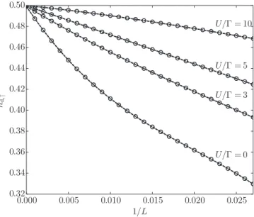
Note, however, that ˆHC does not obey particle-hole sym- metry for finiteL but only in the thermodynamic limit. De- viations from particle-hole symmetry can be monitored by investigating the site occupancy of the impurity. Deviations from the exact value of one-half, see Eq. (19), can be used to quantify the violation of particle-hole symmetry; see Sec.V.
In the numerical renormalization group approach, the SIAM is directly considered in energy space. After an ap- propriate discretization, the resulting Wilson chain is treated numerically [9]. In our approach, we map the Hamiltonian on finiterings to a chain while keeping particle-hole symmetry and the bandwidth finite. The use of a Hamiltonian on a ring geometry permits the direct application, comparison, and assessment of lattice-based variational methods such as Hartree-Fock, Gutzwiller, and DMRG, as done in this work.
Our results also permit us to assess the quality of other present and conceivable future many-body methods for lattice Hamiltonians.
D. Spin correlation function
In this work we visualize the Kondo screening cloud for the single-impurity Anderson model. To this end, we calculate the spin correlation function between the impurity and bath sites.
1. Definition and general properties
Due to the spin-rotational invariance of the model it is sufficient to study the spin correlation function along the spin quantization axis. The local correlation function is defined by
CddS = 0|SˆdzSˆzd|0 = 14 0|( ˆnd↑−nˆd↓)2|0
= 14 −12 0|ˆnd↑nˆd↓|0, (40) where we used particle-hole symmetry (19) in the last step.
The value for the on-site spin correlation interpolates between the itinerant limit,Cdd(U=0)=1/8, and the atomic limit, Cdd(W =0)=1/4.
The correlation function between the impurity site and the bath siteris defined by
CdcS (r)= 0|SˆzdSˆrz,c|0
= 14 0|( ˆnd↑−nˆd↓)( ˆc+r,↑cˆr,↑−cˆ+r,↓cˆr,↓)|0. (41) Due to inversion symmetry we have
CdcS (L−r)=CdcS (r) (42) for 1r(L−1)/2.
To visualize the screening of the impurity spin, we define S(0)=CddS +CdcS (0) and, forR1,
S(R)=CddS +CdcS (0)+ R
r=1
CdcS (r)+CdcS (L−r) . (43) It describes the amount of the unscreened spin at distance R from the impurity site [18]. The impurity is completely screened by all bath electrons. To see this we considerS((L− 1)/2)on finite systems,
S((L−1)/2)= 0|Sˆdz
Sˆzd+
L−1
r=0
Sˆzr,c
|0
= 0|SˆdzSˆz|0 =0, (44) because|0is an eigenstate of the operator ˆSz for the total spin in thezdirection with eigenvalue zero.
2. Spin correlations in two-chain geometry For the first site of the chain we have
CdcS (0)=14
C0( ˆnd↑−nˆd↓)( ˆC0,↑+ Cˆ0,↑−Cˆ0,↓+ Cˆ0,↓)C0 , (45) where we used Eq. (39) and the normalization of|0S.
For the spin correlation function between the impurity site and a bath site at distance 1r(L−1)/2 we use inversion symmetry (42) to write
CdcS (r)= 0|SˆdzSˆzr|0
= 12 0|Sˆdz
Sˆrz+SˆzL−r
|0
= 18
C0( ˆnd↑−nˆd↓)( ˆCr+,↑Cˆr,↑−Cˆr+,↓Cˆr,↓)C0 , (46)
where we used the mapping onto the chain operators in the second step,
ˆ
c+r,σcˆr,σ+cˆ+L−r,σcˆL−r,σ =Cˆr+,σCˆr,σ +Sˆr+,σSˆr,σ, (47) and the factorization (39) in the last step; recall that theS- electron system is a paramagnetic Fermi sea, 0S|Sˆ+r,↑Sˆr,↑− Sˆr+,↓Sˆr,↓|0S =0.
Equations (45) and (46) must be evaluated using DMRG, in general. ForU =0, the ground-state energy and the spin correlation function can be evaluated analytically to a large extent, as we show next.
III. NONINTERACTING SIAM
It is instructive to discuss the noninteracting SIAM. More- over, it provides the basis for the Gutzwiller approach in Sec. IV. We defer the details of the derivation to the Sup- plemental Material [27] and merely summarize the relevant results.
A. Ground-state energy
The ground-state energy sums the band contribution and the energy of the doubly occupied bound state. The total energy reads [27]
e0(V)=eband0 (V)+eb0(V)
= 1 2π
−π+2v+arctan 1
v−
+v−ln
v+−1 v++1
+(1−v+), (48) where
v±(V)≡v±= √
1+64V4±1
√2 . (49) The small-V expansion becomes
esmall0 (V)= 4V2
π [ln(V2)+ln(2)−1]−4V4. (50) Corrections are of the order V6ln(V2). For V =0.1, the approximate formula works very well. We have e0(0.1)=
−0.06291 whereas the approximation gives esmall0 (0.1)=
−0.06294, with a relative error of less than one per mill.
To determine the Gutzwiller variational energy we also need the derivative of the ground-state energy. We have e0(x)= 4x
π[v+(x)2+v−(x)2]
2πv−(x)
arccot[v−(x)]
π −1
+v+(x) ln
v+(x)−1 v+(x)+1
. (51)
For smallxthis reduces to
e0(x1)≈(8x/π) ln(2x2). (52) B. Magnetization and zero-field magnetic susceptibility We introduce the magnetic energy scale Bimp ≡B= (gμB/2)H, where H is the external magnetic field at the
impurity, and express the impurity magnetizationM(V,H)= gμBm(V,B) in terms of the impurity spin in thezdirection,
m(V,B)= Sˆzd
=( nˆd,↑−nˆd,↓)/2. (53) The magnetic susceptibility follows from
χ(V,B)=∂M(H)
∂H =gμB
2
2∂[2m(V,B)]
∂B . (54) We give closed expressions for m(V,B) andχ(V,B) for the noninteracting SIAM in one dimension.
1. Magnetization
For the one-dimensional noninteracting SIAM we find for a magnetic field that acts solely at the impurity [27]
2m(V,B)=Z[vb(V,B)]−Z[vb(V,−B]
+
σn=±1
0
−1/2
dω π
σn√ 1−4ω2 (ω+σnB)2(1−4ω2)+2
(55) with =2V2. Here, vb(V,B)<−1/2 is the energy of the bound state outside the band. It is the root ofP+(ω,B), i.e., P+(vb(V,B))=0, with
P+(ω,B)=ω+B+ 2V2
√4ω2−1. (56) Moreover, the weight of the bound state in the d-electron spectral function is given by
Z[vb(V,B)]=
1− 8V2vb(V,B) {4[vb(V,B)]2−1}3/2
−1
. (57) In general, the magnetization must be determined numerically from Eqs. (55) and (57).
2. Small hybridizations
In the limitV 1, we ignore the bound-state contribution of orderV4, and simplify the magnetization to
m(V,B)= 0
−∞
dω 2π
(ω+B)2+2 − (ω−B)2+2
= B
0
dω π
ω2+2 = 1
πtan−1(B/). (58) The widthof thed-electron spectral function is the relevant energy scale for magnetic excitations.
For small hybridizations, the susceptibility becomes χ(V,B)=gμB
2 22
π
B2+2 (59) with the zero-field limit
χ0(V)=gμB
2 2 2
π. (60)
As seen from Eq. (59), in the limitV →0 the magnetic sus- ceptibility is proportional to the zero-fieldd-electron spectral function,μ(V,B)∝Dd,d,σ(B) [27].
3. External magnetic field for impurity and bath electrons For the caseBimp=Bbath≡B, the bound states are shifted in energy,
vb(V,B)= −B−v+(V)/2, (61) but their weights Z[vb(V,B)] do not change because vb(V,±B)±B= −v+(V)/2 in both cases. The rigid shift in single-particle energies by the magnetic field also guarantees that the impurity remains half filled on average for all external fields. The impurity magnetization becomes (BW)
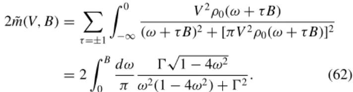
2 ˜m(V,B)=
τ=±1
0
−∞
V2ρ0(ω+τB)
(ω+τB)2+[πV2ρ0(ω+τB)]2
=2 B
0
dω π
√ 1−4ω2
ω2(1−4ω2)+2. (62) For small hybridizations, ˜m(V,B) reduces to the result for m(V,B) in Eq. (58).
We show the impurity magnetization as a function ofB/
in Fig.2. Only forV =0.2 andB2, there is a discernible difference between the curves form(0.2,B), Eq. (55), where the external field is confined to the impurity, and ˜m(0.2,B), Eq. (62), where the external field polarizes all electrons. In both cases, the DMRG data, see Sec.V, faithfully reproduce the analytic results, within small errors resulting from finite- size effects.
The wide-band limit closely follows the result for the global magnetic field. This indicates that the difference be- tween applying the external field locally or globally is mostly due to the polarization of the bound states for a local field. The bound states have a noticeable weight forV =0.2.
FIG. 2. Impurity magnetization for the noninteracting symmet- ric SIAM for V =0.2 as a function of B=gμBH/2. We show m(0.2,B), Eq. (55) (local field, blue dotted line), ˜m(0.2,B), Eq. (62) (global field, red straight line), and the wide-band limit (58) (local field, black dashed line), together with the corresponding DMRG data (symbols, L=997 sites). Inset: Impurity magnetization for V =0.1.
Since the weight of the bound states is of the orderV4, their contribution is much smaller forV =0.1. Correspondingly, as seen from the inset of Fig. 2, the discrepancies between the magnetization curves for local and global external fields become very small. Since we shall work withV 0.1 for the rest of the paper, we will restrict ourselves to purely local external magnetic fields, and shall safely ignore the influence of the magnetic field on the bath electrons.
C. Spin correlation function 1. General properties
Starting from Eq. (41) we can use Wick’s theorem and spin symmetry to show that
CdcS (r)= −21| 0|cˆ+r,↑dˆ↑|0|2≡ −12Mr2 (63) for the ground state |0 of the noninteracting SIAM.
The matrix element is calculated in the Supplemental Material [27],
Mr = 1
L
k
e−ikr 0|cˆ+k,↑dˆ↑|0
=V π
0
dk
π cos(kr)M[−cos(k)/2], (64) where we took the thermodynamic limit and used (k)=
−cos(k)/2 in one dimension. SinceM() is real, particle-hole symmetry leads toM(−)=M() so that the matrix element vanishes for odd sites,M2m−1=0,m1. For even sites we find the bound-state and band contributions [27]
M2mb = −2V Z(V)
v+2 −1 (
v+2 −1+v+)−2m,
M2mband = −2V(−1)m π
π
0
dy cos(y/2) sin2(y)+64V4
×[sin(y) cos(my)+8V2sin(my)] (65) with the pole frequencyωb= −v+/2 and the pole weight
Z(V)= 1
1+4V2v+/v3−, (66) andv±from Eq. (49).
2. Small hybridizations
The bound-state contribution Mrb is of the orderV3 for smallV, and becomes exponentially small forr1/(4V2).
For smallV [17], the band contribution is dominated by the regiony→0 in the integrand in Eq. (65). We thus approxi- mate for smallV
M2m≈ −2V π
∞
0
dxxcos(8V2mx)+sin(8V2mx) x2+1
=(−1)m2V
π eαEi(−α), α=8V2m, (67) where
Ei(x)= − ∞
−x
dte−t
t (68)
101 102 r 10−6
10−5 10−4 10−3 10−2
−Cdc(r)
asymptotic exact
0 2 4 6 8 10 12 14 r
0.00.5 1.01.5 2.02.5 3.03.5×10−2
approximation
approximation
exact
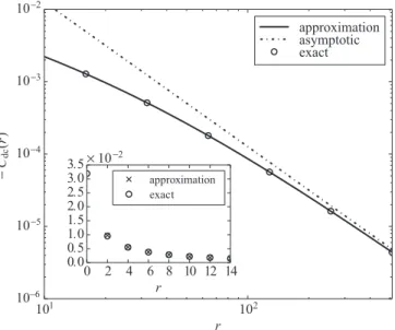
FIG. 3. Spin correlation function for the one-dimensional nonin- teracting symmetric SIAM forV =0.1 (circles) on a log-log scale.
The analytic result (69) is shown as a straight line. The asymptotics (70) is shown as dash-dotted line, and the exact values (65) are shown as open symbols. Inset: Spin correlation function for small distances on a linear scale.
is the exponential integral. Thus, the spin correlation function approximately becomes (m=0)
CdcS (2m)≈ −1 2
2V
π eαEi(−α) 2
, α=8V2m. (69) In Figs.3and4we show the spin correlation function and the unscreened spin for the noninteracting symmetric SIAM
FIG. 4. Unscreened spinS(r) at distance r from the impurity site, see Eq. (43), for the one-dimensional noninteracting symmetric single-impurity Anderson model forV =0.1. The analytic result based on Eq. (69) is shown as a solid line. The asymptotic result (72) is presented by a dotted line. The DMRG data forL=197,1397 sites are given by dashed lines; see Sec.V. Inset: Unscreened spin for small distances; DMRG data forL=1397 sites.
in one dimension forV =0.1. As seen from Fig.3, the spin correlation function decays to zero proportionally to 1/m2. The exact result (65) and the approximate formula (67) yield almost identical results, already form2. Form10, the relative error is of the order 10−4forV =0.1.
Correspondingly, the unscreened spin shown in Fig.4de- cays to zero proportionally to 1/m. For smallV, the screening is fairly inefficient and, correspondingly, the screening cloud extends very far into the host metal, even in the case of the noninteracting SIAM.
3. Small hybridizations and large distances
Here, we work out the long-range behavior of the spin correlation function. The asymptotic regime is reached for α1, i.e., form1/(8V2), where exp(α)Ei(α)≈ −1/αin Eq. (69). For the correlation function we find in this region
CdcS (2m1/(4V2))≈ −1 2
2V πα
2
= − 1 32π2V2
1 m2. (70) For the noninteracting symmetric SIAM in one dimension, the spin correlations between the impurity and a bath electron at site 2masymptotically decay proportionally to 1/(2m)2; see Fig.3.
The matrix element M2m atα=1 [2m=1/(4V2)] is al- ready very small, of the orderV2 in the asymptotic region.
Nevertheless, the contribution to the screening is finite even forV →0. The spins for |m|>1/(8V2) (α >1) contribute approximately
S Cdd
≈8 2V
π
2 ∞
1/(8V2)
dm[eαEi(−α)]2
= 4 π2
∞
1
dα[eαEi(−α)]2≈0.23. (71)
The sites for|m|>1/(8V2) contribute about 25% to the total screening of the spin at the impurity site, whereCdd =1/8.
Indeed, for large distancesr=2mfrom the impurity, the unscreened spin decays only proportionally to 1/r,
S(r1)∼ 1 16π2V2
1
r, (72)
as follows from Eq. (44) when we employ the Euler- Maclaurin formula for the asymptotic expression (70). This is shown in Fig.4.
IV. GUTZWILLER VARIATIONAL APPROACH In this section we define the Gutzwiller variational state and determine its variational parameters from minimizing the variational ground-state energy [23,24]. Moreover, we deter- mine the variational magnetization, zero-field susceptibility, and spin-spin correlation function between the impurity site and the host electrons.
A. Ground-state energy 1. Definition
The Gutzwiller wave function for the symmetric SIAM reads
|G =[λd(nˆd↑nˆd↓+(1−nˆd↑)(1−nˆd↓))+λσ(nˆd↑(1−nˆd↓) +(1−nˆd↑) ˆnd↓)]|0, (73) where|0is a normalized single-particle product state.
The Gutzwiller wave function is normalized,
G|G =1, (74)
and symmetric,
G|nˆd,σ|G = 12, (75) if we use a symmetric single-particle product state,
0|nˆd,σ|0 = 12, (76) and if we set
λ2d =1−
1−q2, λ2σ =2−λ2d =1+
1−q2. (77) Here, we introduced the remaining variational parameter 0 q1 that characterizes the Gutzwiller wave function.
2. Optimizing the variational parameters
The Gutzwiller variational ground-state energy with re- spect to the energy of the bare band is the minimum of
Evar(q)=e0(qV)+U 4(1−
1−q2) (78) over the variational parameter 0q1. Here,e0(V) is the ground-state energy of the noninteracting symmetric SIAM, Hˆ0in Eq. (2); see Eq. (48). The minimum cannot be obtained analytically in general but we can derive an implicit equation.
The minimization condition [dEvar(q)]/(dq)=0 leads to the equation
U(q,V)= −2
1−q2e0(qV)/(qV) (79) with=πρ0(0)V2=πd0V2 =2V2on a chain with nearest- neighbor hopping. Therefore, we know U(q,V) for every 0q1. The variational ground-state energy is thus given implicitly by Eq. (78).
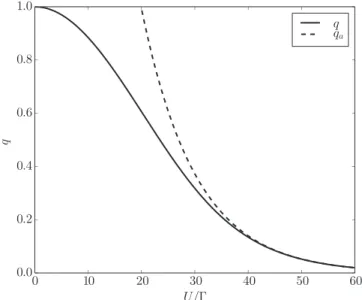
In Fig.5we show the Gutzwiller parameter as a function ofU/forV =0.1, and compare to the analytic expression in the strong-coupling limit.
3. Strong-coupling limit
For strong couplings, we findq→0 so that we may use the small-V expression to derive the variational ground-state energy analytically. Using Eq. (52) in Eq. (79) givesq(U)≈ qa(U) with
[qa(U)]2= 1 exp
−πU 16
, (80)
and the variational ground-state energy becomes Eopt(q1,V)≈ −2
π exp
−πU 16
∝exp
− 1 4d0JK
(81)
40
0 10 20 30 50 60
U/Γ 0.0
0.2 0.4 0.6 0.8 1.0
q
qqa
FIG. 5. Optimal Gutzwiller variational parameter as a function of U/ for V =0.1 and the one-dimensional symmetric SIAM (=πd0V2=2V2). The asymptotic result (80) is shown with a dashed line.
with the Kondo energyJK=4V2/U.
The ground-state energy becomes exponentially small, cor- responding to the exponentially small Abrikosov-Suhl reso- nance in the spectral function [3]. However, the Gutzwiller ex- ponent is too small by a factor of two,TK∝exp[−1/(2d0JK)]
[3]; i.e., the Gutzwiller approach overestimates the width of the resonance. As seen from Fig.5, forV =0.1 the asymp- totic behavior sets in aroundU/≈35, forq0.2.
B. Magnetization and magnetic susceptibility
In the Gutzwiller variational approach, the impurity spin in thezdirection is given by
mG(V,B)= λ2σ
2 0|nˆd,↑−nˆd,↓|0 (82) withλσ from Eq. (77). Here, we keep a spin-independentq factor and only consider the magnetic-field-induced changes in the single-particle product state |0. Therefore, the Gutzwiller variational result for the magnetization can be obtained from the noninteracting expression by replacing q withqV, see Sec.III B,
mG(V,B)=(1+
1−q2)m(qV,B). (83) The zero-field susceptibility in Gutzwiller theory reads
χ0G(V,U)=(1+ 1−q2)
gμB
2 2 2
π 1
q2 (84) so that the variational Wilson ratio becomes
RG(V,U)= χ0G(V,U)
(gμB/2)2DGd,d(ω=0) =1+
1−q2. (85) Here, we used the fact that the Gutzwiller approach describes a Fermi liquid in which the density of states at the Fermi level is enhanced by a factor 1/q2. Equation (85) shows that the Gutzwiller approach correctly reproduces the weak-coupling