Gergely Zar´and Quantum Impurity Problems Work presented to obtain the title ’Doctor of the Hungarian Academy of Sciences’ Budapest University of Technology and Economics Budapest, 2005

(1)

Gergely Zar´ and

Quantum Impurity Problems

Work presented to obtain the title

’Doctor of the Hungarian Academy of Sciences’

Budapest University of Technology and Economics

Budapest, 2005

(2)

(3)

1 Introduction

Quantum impurity models have continuously been in the focus of intense research in the past 50 years. While the expression designating this class of models indicates that these models were originally constructed to describe the quantum mechanical properties of an impurity or imperfection such as a magnetic atom, dislocation, or a substitutional ion in a lattice, in reality, the history of these models dates back to the very early days of quantum mechanics, when the quantum mechanics of the electron spin and magnetic ions in an external magnetic field and the tunneling of a particle in a double well potential (two level system) have been worked out.

The behavior of an isolated spin or two level system is, of course, trivial. However, their physics becomes extremely complex once one considers them as ’impurities’, i.e., once one takes into account that they couple to excitations in the environment.

In fact, quantum impurity models represent the simplest non-trivial quantum field theories which, despite of their simplicity, provide the simplest examples of exciting phenomena such as quantum criticality, dynamical mass generation, asymptotic freedom, duality, or universality. Besides being interesting on their own, quantum impurity models also serve as a test ground for more complicated strongly correlated lattice systems that occur in nature. As an introduction to this thesis, let me give here a short overview of some of the most important milestones in the theory of quantum impurity problems to introduce the reader into this exciting field.

1.1 The Kondo effect

The complexity of the problem of coupling a quantum mechanical degree of freedom to a dissipative environment has been probably first realized by Kondo, who proposed to describe the interaction of a magnetic impurity and the conduction electrons by the following simple Hamiltonian [1]

Hint = J 2

X

k,k^′,σ,σ^′

S c~ ^†_kσ~σσσ^′ck^′σ^′ , (1)

where J > 0 denotes the antiferromagnetic coupling between the impurity spin S~ and the conduction electron spin density at the origin, and the operator c^†_kσ creates a conduction electron with momentum k and spin σ. Kondo discovered that the simple Hamiltonian Eq. (7) - called the Kondo model after Kondo - gives rise to a

(6)

logarithmic increase in the resistivity at low temperatures. However, while the theory of Kondo successfully explained the low-temperature resistivity anomaly observed in various magnetic alloys, it also alerted physicists: the seemingly innocent and simple Kondo model contains infrared singularitieswhich make it impossible to understand the low-temperature properties of this model by simple perturbation theory, that breaks down at the so-called Kondo temperature,

TK ≈EF e⁻^1/J̺⁰ . (2)

In the above expression EF denotes the Fermi energy, and̺0 is the density of states of the conduction electrons at the Fermi level for a given spin direction.

One of the major steps in understanding the Kondo model was made by Anderson and his coworkers [3, 4]. First Anderson, Yuval, and Hamann used renormalization group (RG) techniques to study the strongly anisotropic version of Eq. (7)

Hint = J_⊥ 2

X

kk^′

(c^†_k_↑ck^′↓S⁻+ h.c.) + J_k 2

X

kk^′

(c^†_k_↑ck^′↑−c^†_k_↓ck^′↓)S^z , (3) where the coupling in the z-direction is much larger than the one in the x, y directions, J_k ≫J_⊥. Anderson, Yuval and Hamann expanded the free energy functional of this model as an imaginary time path integral by treating J_⊥ as a perturbation, and mapping it to the one-dimensional Coulomb gas: spin flips behave as charged particles after the mapping and interact through a logarithmic interaction in time.

The scaling analysis of Anderson et al. showed that the amplitude of spin-flip pro- cesses increases as one lowers the temperature, and ultimately dominate the low temperature physics [3].

Later Anderson proposed a much simpler version of renormalization group analysis, the so-called ’poor man’s scaling method’, where the elimination of high-energy conduction electrons has been compensated by changing the value of the dimensionless coupling, ̺0J, while keeping matrix elements of the T-matrix in the vicinity of the Fermi surface invariant [4]. Anderson’s scaling approach can be shown to sum up the most singular diagrams in the perturbation series, first identified by Abrikosov [5], and it breaks down at the Kondo scale (2), where the effective coupling obtained diverges. Anderson believed that this is an artifact of the approach, and conjectured that the effective coupling diverges only in theT →0 limit. The divergence of the effective coupling could be formally cured by extending Anderson’s method to sum up

(7)

subleading diagrams and casting in the form of multiplicative renormalization group, though the results of these perturbative renormalization group calculations remained consistent only above (a somewhat reduced) T_K, where the effective coupling was much less than unity [6, 7, 8]

The real break-through in understanding the low-temperature behavior of the Kondo problem came from Nozi`eres [9], who took the divergence of the effective coupling seriously, and showed by an expansion in 1/J that theJ =∞fixed point is indeed stable. He also identified the leading corrections around theJ → ∞limit, and showed that at low temperatures the Kondo model becomes a ’local Fermi liquid’, with weakly interacting quasiparticles at the impurity site, and derived the behavior of resistivity and thermodynamic quantities. In other words, the impurity spin forms a singlet state with the conduction electrons at low temperatures, and completely disappears from the problem. A quantitative understanding of the Kondo problem has been finally achieved by Wilson who - in the spirit of renormalization group - proposed a numerical scheme (discussed in Section 2.3 of this thesis) to diagonalize the Kondo Hamiltonian iteratively [10]. With this method, he was able to compute thermodynamic quantities at all temperatures, and he has also been able to deduce the renormalization group flow of the effective coupling, and confirm Anderson’s conjecture and Nozi`eres Fermi liquid picture.

The solution of the Kondo problem, however, did not end with the work of Wilson: five years after Wilson’s work a complete Bethe ansatz solution of the Kondo problem was constructed [11, 12, 13], but one had to wait another fifteen years until it became also possible to compute dynamical correlation functions and the resistivity numerically with a high accuracy [14, 15].

Parallel to the efforts to understand the Kondo model, the problem of magnetic impurities has been attacked from another direction as well. In 1961 Anderson proposed a more detailed model to describe the formation of magnetic moments on the d-level of rare earth metals [16]. Anderson showed that if the interaction energy U of the d-electrons is strong enough compared to the hybridization energy Γ then, in general, a magnetic moment will be formed on the d-level. Later, Schrieffer and Wolff constructed a unitary transformation and showed that, for small values of Γ/U and small enough energy scales, the physics of Anderson’s model is practically equivalent to that of the Kondo model in the local moment regime [17]. A year after Nozi`eres’ Fermi liquid theory, Yamada and Yosida published a series of papers [18],

(8)

where they showed that perturbation theory in the Anderson model is convergent, and the low temperature properties are that of a Fermi liquid. In a way, the results of Yamada and Yosida were the logical extensions of the general theory of Luttinger [19, 20].

Based on the above results, we now understand the Kondo effect as follows (see Fig. 1): Due to the strong coulomb interaction, a local moment is formed on the deep d or f-levels of rare earth and actinide materials. This local moment is essentially free at temperatures T > TK, and its susceptibility - apart from small logarithmic corrections - increases as χimp ∼ 1/T for T > TK. However, as we lower the temperature, the system tries to get rid of the high temperature entropy of the spin, S =kBln(2S+ 1), and a conduction electron spin is bound to the impurity antifer- romagnetically to screen the impurity spin and form a local singlet. The energy of this many-body state is given by the Kondo energy TK. Since a finite energy ∼ TK

is needed to break up this singlet, conduction electrons at the Fermi energy are not allowed to enter the impurity site and correspondingly, scatter off elastically with a phase shift π/2, and the impurity contribution to the susceptibility is finite at low temperatures, χimp ∼1/TK.

T > T

_K

T < T

_K

J = 0 J = infty

Figure 1: renormalization group flow of the effective coupling and the the formation of the corresponding local singlet in the single channel Kondo model.

1.2 Dissipative two level systems

One of the most important and most interesting quantum impurity problems is that of a dissipative two level system (TLS). This model has been maybe first proposed by Leggett in the context of macroscopic quantum tunneling [21, 22], who studied how coupling to a dissipative environment destroys the quantum-coherent motion of

(9)

a two state system. Leggett proposed to study the simplest non-trivial model one can envision, a tunneling system coupled to a bath of harmonic oscillators:

HSB =−1

2∆τx+1

2ετz+^X

i

ωi(a^†_iai+1 2) + 1

2τz

X

i

Ci

√2miωi

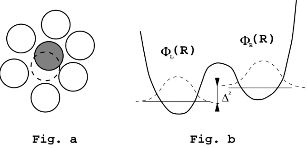
(ai+a^†_i). (4) Here τi, i= x, y, z are Pauli spin matrices, the two states of the system correspond to τz =±, ∆ is the bare tunneling matrix element and ε is a bias.¹ The harmonic oscillators are labeled by the indexi, have masses m_i and frequenciesω_i, and couple linearly to the coordinateQ= ¹₂τz of the two level system with couplingsCi. Eq. (4) being quadratic in the oscillator coordinates, one can integrate out the bosonic degrees of freedom, and finds that the dynamics of the spin operators is uniquely determined by the oscillators’ spectral function J(ω) = ^π₂ ^P_i(_m^Cⁱ²

iωi)δ(ω−ωi).

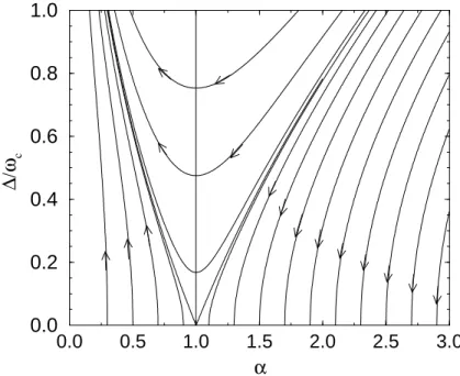
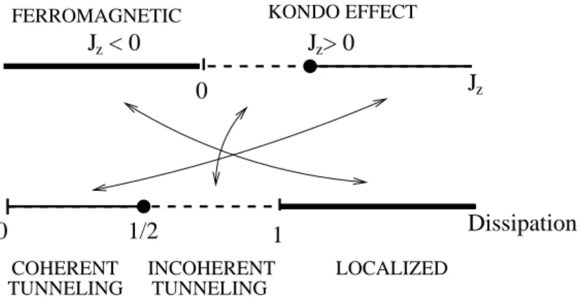
Maybe the most interesting case is that of an Ohmic heat bath, where J(ω) is linear below a high frequency cut-off ωc, J(ω) = 2παω. In this case, as we shall discuss in Section 3.1.3, increasing dissipation strength α first makes the motion of the tunneling particle incoherent, and for α > 1 dissipation can even completely suppress tunneling and localize the tunneling particle [22]. Remarkably, there is an exact mapping outlined in Section 3.1.2, which maps the above basic model of dissipation on the anisotropic Kondo model, Eq. (3) [22, 23]. This mapping connects the parameters of the two models as

∆ ωc

= ̺0J_⊥ ≡j_⊥ (5)

α = (1− 2δ

π )², (6)

whereδ= arctan^πρJ₄^k is the scattering phase shift for conduction electrons generated by the potential J_k/4, and the bias ε in Eq. (4) corresponds to a local magnetic field in the Kondo problem. This surprising result implies that many dynamical properties of the two models and their thermodynamics are completely equivalent, and essentially all dissipative physics is contained in the anisotropic Kondo problem.

1Throughout this dissertation we use units ¯h=k_B =µ_B = 1. In many cases we also set the Fermi velocity tov_F = 1.

(10)

1.3 Non-Fermi liquid models

In the eighties another new class of fascinating quantum impurity problems chal- lenged theoretical physicists. In 1980 Nozi´eres and Blandin attempted to construct realistic models for magnetic impurities,i.e., to take into account crystal field effects properly [24]. Under special circumstances they found that the coupling between the magnetic moment and the conduction electrons is described by a multichannel version of Eq. (7)

Hint = J 2

X

σ,σ^′,a

S ψ~ ^†_σa~σσσ^′ψσ^′a, (7) where the channel quantum numbera= 1, .., f isconservedin course of the scattering process. The variant of this model with spin S = 1/2 and f = 2 is the so-called two-channel Kondo model.

T > T

_K

J = 0 J

^*

J = infty

= =

....

T < T

_K

Figure 2: Renormalization group flow of the effective coupling in the two-channel Kondo model. No singlet can be formed because of the symmetry of the two channels, and an intermediate coupling fixed point governs the T →0 physics.

Nozi`eres and Blandin realized that this model must have properties very different from the usual spin S = 1/2 Kondo problem, as can be understood by simple renormalization group arguments: similar to the Kondo problem, for small values of j = ̺0J the effective coupling increases under the renormalization group transformation, suggestive of a strong coupling fixed point. However, the j → ∞ fixed point of the RG is unstable: For j =∞ the impurity spin would bind a conduction electron from each channel, thus giving a local residual spin ˜S = 1/2. This residual spin couples to the rest of the system through an antiferromagnetic exchange coupling of size ˜j ∼ 1/j. This coupling is again relevant, implying that for very large values of j, ˜j must increase and thus j must decrease under the RG (see Fig. 2).

These arguments imply that the effective low energy theory has a finite exchange

(11)

couplingj^∗, and is not trivial. As a consequence, the model has a residual entropy at T = 0 temperature, the susceptibility and the linear specific heat coefficient diverge asT →0 [25, 26], and the resistivity shows a power-law anomaly [27]. Furthermore, Maldacena and Ludwig showed that quasiparticles at the Fermi energy are orthogonal to conduction electrons [28], and an incoming electron at the Fermi surface

’evaporates’ and scatters to infinitely many electron-hole excitations.

Nozi`eres and Blandin realized that non-Fermi liquid states are extremely fragile, and therefore they did not really believe in the existence of realizations of these exotic models [29]. It came therefore as a surprise when D.L. Cox suggested that many of the logarithmic anomalies in Uranium and Cerium based heavy fermion compounds can be explained in terms of the two-channel Kondo model, and showed that the two-channel Kondo model naturally shows up as a consequence of the crystal field structure of these materials [30, 31]. The most important ingredient of these models is the strong spin-orbit coupling at the deepf-levels of Uranium and Cerium, originally not considered by Nozi`eres and Blandin.

Since then, a few other realizations of non-Fermi liquid systems have been proposed such as non-commutative two level systems [32, 33, 34], quantum dots in the vicinity of their degeneracy point [35], and multi-dot systems [36], some of which will be also discussed in this thesis.

1.4 New Directions

To close this Introduction, let us discuss a few more recent applications of quantum impurity models.

1.4.1 Heavy Fermion physics, strongly correlated systems, and quantum critical points

One of the major challenges of today’s solid state physics is to understand strongly correlated heavy fermion systems and strongly correlated systems such as high temperature superconductors or manganites. Heavy fermion compounds are usually (seemingly) complicated Cerium or Uranium-based alloys, where much of the physical properties is governed by the f-electrons on the Ce and U ions. These ions usually form a dense lattice, and provide local moments at high temperature which are screened by the conduction electrons as one lowers temperatures. At these low temperatures, the f electrons form a narrow resonance (Kondo resonance) at the

(12)

Fermi level which gives the dominant contribution to the specific heat and the susceptibility, corresponding to an effective mass 100−1000-times larger than the free electron massm_e.[2, 34] It is for this reason that we call these systems heavy Fermion systems or heavy Fermi liquids.

Surprisingly, many of the thermodynamic properties of these systems could be qualitatively understood in terms of single impurity physics [34]. To obtain a better understanding, however, more elaborate methods are needed. One of the most efficient methods is the so-called dynamical mean field theory in which one keeps local time-dependent correlations, but spatial correlations are treated only at the mean field level [37, 38]. This theory becomes exact in the limit of infinite coordination number, and entails solving a quantum impurity problem, where the conduction electrons’ spectral function is determined self-consistently. Therefore, having a deep understanding of quantum impurity problems is essential in understanding phenomena such as the Mott metal-insulator transition. There is currently a major effort in combining dynamical mean field theory with usual band theoretical methods to keep track of correlations, however, efficient impurity solvers still need be developed to achieve this goal.

As mentioned before, in heavy Fermion compounds the conduction electrons screen out the magnetic moments at low temperatures. This is, however, not the only way to get rid of the residual entropy of the local moments: the conventional way to get rid of the residual entropy in a magnetic material is through the formation of a magnetically ordered state. In fact, in most heavy Fermion systems these two mechanisms compete with each other, and depending on the ratio of exchange coupling between neighboring ions and the Kondo temperature one or the other prevails. The before-mentioned ratio can be fine-tuned by pressure, impurity concentration, or magnetic field to lead to a transition from a non-magnetic metal state to a magnetically ordered metal [39, 40, 41, 42, 43, 44, 45]. In many cases this T = 0 temperature transition is of second order, and the corresponding transition is a quantum phase transition governed by quantum fluctuations [46]. In some systems neutron scattering data are suggestive of a quantum critical point that can be described in terms of local quantum fluctuations, i.e., some quantum impurity models [41]. One of the most prominent candidates to describe these locally quantum critical systems is the Bose-Fermi Kondo model, and shall be analyzed in Section 3.3 of this dissertation.

(13)

Finally, another open question to answer is the origin of heavy Fermion super- conductivity. In many heavy Fermion systems the heavy electrons become superconducting at low temperature and usually form a non-conventional superconducting condensate with gapless nodes or lines at the Fermi level [34]. The mechanism to form this superconducting state is almost certainly provided by local quantum fluctuation-generated correlations, which probably also determine the symmetry of the superconducting state. This is a fascinating possibility that has never been care- fully studied before, probably because of the difficulty of the problem. With the fast development of numerical methods, however, it appears to be possible to study these phenomena in the near future by combining dynamical mean field theory with other approaches.

1.4.2 Mesoscopic systems: Building artificial atoms from electrical circuits

With the recent development of lithography it became possible to design and build electronic circuits in a controlled way with sizes down to the µ range and below.

The energy needed to put an electron to such a small island is roughlyEC ∼e²/d∼ 10⁻³eV∼10K,i.e. it can be larger than the temperature of the device. Under these conditions the island operates as an ’artificial atom’ [47]. One can also build ’artificial molecules’ by joining several ’artificial atom’, attach them to leads to measure transport properties and the effect of quantum fluctuations and change the number of electrons on them by simply varying gate voltages.

One can also engineer narrow constrictions (point contacts or nano-wires), al- lowing one to measure the dynamical properties of individual atoms [71]. Similar to single electron transistors, these point contacts can also be used as voltage probes or amplifiers in nanoscale circuits.

Quantum impurity models proved extremely useful in mesoscopic physics, since much of these systems including single electron transistors, metallic islands, or Josephson qubits (being maybe the most promising candidates for quantum computing) can be described in terms of them.

Mesoscopic technology also makes it possible to study out of equilibrium transport properties of these ’artificial’ atoms in an unprecedented way, and many unex- pected strongly correlated states have been observed in this way [48, 49, 50, 51, 135].

More recently, it became also possible to contact real molecules, and perform ex-

(14)

periments on them [118]. The experiments are performed in many cases out of equilibrium. The complete understanding of these mesoscopic and nanoscopic circuits with strong correlation effects represents therefore a major challenge for todays’

theoretical physicists, and represents an unsolved problem of this field [54, 56, 55].

In this effort quantum impurity problems serve as a test ground, but combining quantum field theoretical techniques to study transport through molecules is still a dream.

1.5 Structure and subject of the dissertation

The purpose of this dissertation is to review some of the results obtained by the author in the field of quantum impurity problems. First, in Chapter 2 I give a short review of the theory of Kondo effect and introduce some of the methods I shall use to study quantum impurity models later, such as multiplicative renormalization group, numerical renormalization group, and Bethe ansatz.

In Chapter 3 I study dissipation effects. First I introduce and analyze using various methods the most basic Ohmic dissipative two level system model in Section 3.1.

Then in Section 3.2 I study the same system by numerical renormalization group methods in the case when the tunneling particle has a spin. The last section of this chapter is devoted to theǫ-expansion study of the Bose-Fermi Kondo problem, where both dissipative bosonic fields and conduction electrons couple to an impurity spin.

Chapter 4 is devoted to various non-Fermi liquid models and the discussion of their physical realizations. First in Section 4.1.1 I show using 1/f expansion methods how the physics of fast two level systems maps on the two-channel Kondo problem.

Then in Sections 4.1.2 and 4.1.3 I study the anisotropic Kondo model using Abelian bosonization and Bethe ansatz methods. In the last two sections of the chapter, Sections 4.2.1 and 4.2.2, I generalize the mapping discussed in Section 4.1.1 to the case ofM-state systems, and then solve the corresponding Coqblin-Schrieffer model by Bethe ansatz techniques.

Finally, in Chapter 5 I study mesoscopic systems. After giving a short introduction to the theory of single electron transistors, in this chapter I analyze phenomena such as the singlet-triplet transition, the SU(4) Kondo effect, quantum fluctuations of a ferromagnetic grain, and study magnetic impurities in point contacts.

Section 3.1.4, Section 3.2, Section 3.3, Section 4.1.1, the second part of Sec- tion 4.1.2, Section 4.1.3, Section 4.2, Section 5.1.3, Section 5.1.4, and Section 5.2

(15)

contain mostly or exclusively my own results.

(16)

2 The single channel Kondo problem

The Kondo model given by Eq. (7) is one of the most elementary quantum impurity problems, and much of our understanding of other quantum impurity problems relies on our experience with it and the methodology that has been used to study it. We shall therefore start by reviewing part of the theory of Kondo model in this chapter.

2.1 Renormalization group analysis

2.1.1 Poor man’s scaling

As mentioned in the introduction, the Kondo model contains infrared singularities.

This can be seen most easily if one computes the on-shell matrix elements of the many-body T-matrix at T = 0 temperature between single electron states, |ini = c^†_k′σ^′|s^′iand|outi=c^†_kσ|sidoing perturbation theory in Eq. (7). Here|sidenotes the filled Fermi see (vacuum) with the impurity spin in state S^z = s. Straightforward second order perturbation theory yields [1]

hout|Tˆ|ini ≈ J

2S~ss^′~σσσ^′(1 +J̺0lnD

ω +. . .), (8)

where ω is the energy of the incoming electron (or hole) measured from the Fermi energy, andDis a bandwidth cut-off of the order of Fermi energy. Clearly, the second order term diverges asωapproaches the Fermi energy. This infrared divergence is due to intermediate electron states with arbitrarily small energies, and is characteristic of almost all quantum impurity problems where an impurity is coupled to the Fermi sea.

Higher order contributions can be most easily computed using Feynman diagrams, and can be classified according to their leading singularity [5]. In general, the most singular order n corrections to the T-matrix diverge as ∼Jⁿ⁺¹ln^{n D}_ω, and correspond to a special subset of diagrams, the so-called parquet diagrams. These diagrams can be explicitly summed up and give the following result,

hout|̺0Tˆ|ini^leading = 1

2S~ss^′~σσσ^′t(ω), t(ω) = ̺0J

1−J̺0ln^D_ω = 1

ln^T_ω^K , (9) where the Kondo temperature defined by Eq. (2) has been introduced and t(ω) is the dimensionless T-matrix. Most disturbingly, the sum of the leading logarithmic

(17)

diagrams diverges at TK.

Anderson provided a much simpler way to sum up these most divergent contributions [4]. One only has to assume that the physical properties of the Kondo model are not sensitive to the high-energy cut-off D, and the only energy scale that enters is the dynamically generated scaleTK, as also suggested by Eq. (9). In other words, one can reduce the cut-offD in Eq. (9) and compensate it by rescaling the exchange coupling J such that all physical (measurable) quantities remain constant. In the language of particle physics, this simply means that the theory is renormalizable, i.e. that one can remove the cut-off from the problem through a renormalization procedure [57]. With this assumption one can immediately derive solely from Eq. (8) the dimensionlessT-matrixt(ω) as follows: Clearly, to keep the dimensionless quan- tity hout|̺₀Tˆ|ini constant, one must change the value of J in the following way to compensate the reduction of the cut-off, D→D^′,

D→D^′ , J →J^′ =J+J²̺0ln D

D^′ +. . . . (10) For infinitesimal transformations this equation can be cast in the form of a differential (or scaling) equation, originally constructed by Gell-Mann and Low

∂j

∂l =β(j), (11)

where β(j) = j²+. . . is the beta function, j(l) = ̺0J(D) the renormalized dimensionless coupling,D0is the original cut-off, and we introduced the logarithmic energy scale l = ln^D_D⁰.

To obtain the effective coupling for an equivalent model with band-width D one has to integrate Eq. (11) up tol= ln^D_D⁰ with the initial conditionj(l= 0) =j₀. This invariance can be used to determine physical quantities in a very efficient way if we observe that in a theory with cut-offD≡ω the logarithmic terms identically vanish, and physical quantities are thus given by the leading order (non-logarithmic) diagrams. The dimensionlessT-matrix,e.g. can be immediately obtained from Eq. (11) using t(ω) = j(l = lnD0/ω) in this way. Leading singularities of thermodynamic quantities and the resistivity can be obtained in a similar way, by exploiting the fact that all physical (measurable) quantities are invariant under the renormalization group (RG) transformation.

(18)

2.1.2 Multiplicative Renormalization Group

Although possible, it is not very easy to generalize the method of Anderson to sum up subleading singularities, which correspond to higher order terms in the beta function on the r.h.s of Eq. (11) [6]. A more efficient way to do this was invented independently by Fowler and Zawadowski and Abrikosov and Migdal [7, 8], who used field theoretical renormalization group methods to derive the scaling equations. The essence of this technique is to represent spin states by pseudofermions as|Sz =si ↔ b^†_s|0i and the spin operator as [5]

S~ →^X

s,s^′

b^†_sS~ss^′bs^′ , ^X

s

b^†_sbs≡1. (12) The latter constraint can be enforced by introducing a chemical potential λ for the pseudofermions and then collecting leading contributions ∼e⁻^βλ asλ → ∞.

The theory is then formulated in terms of the electronic Green function,G(ω, ξ(k)), the pseudofermion Green function, G(iω, ξ(k)), and the pseudofermion-conduction electron vertex function Γ({ω_i}), where {ω_i} denote the external Matsubara frequencies of the pseudofermions and the electrons, respectively. Implicitly, all these functions depend on the high energy cut-off D and the dimensionless coupling j.

Similar to poor man’s scaling, the multiplicative renormalization group scheme provides connection between equivalent physical systems with different parameters but the equivalence is formulated as an internal symmetry of the Green’s functions. The main assumption of of the multiplicative renormalization group is that the Green’s functions and vertex functions of the original and the renormalized problem have the same functional form, apart from overall multiplicative factorsZe and Z, which are independent of ω [7, 8]

G(ω, D^′, j^′) =Ze(D^′/D, j)G(ω, D, j), (13) G(ω, D^′, j^′) = Z(D^′/D, j)G(ω, D, j), (14) Γ(ω, D^′, V^′) = Z_e(D^′/D, j)⁻¹Z(D^′/D, j)⁻¹Γ(ω, D, j), (15) where the primed parameters are those of the renormalized system, and the renormalized electron- and pseudofermion Greens functions are given by

G= (iω−ǫ−Σe(ω))⁻¹ , (16)

(19)

G = (iω−λ−Σ(ω))⁻¹ , (17) with Σe(ω) and Σ(ω) the electrons’ and the pseudofermion’s self-energy. Note that the multiplicative prefactors do not contain the dynamical variables ω, and that the prefactor of the vertex function and the two Green’s functions are related (see Eq. (15)). This latter relation is necessary to ensure that the singular part of the free energy remain invariant. Again, the connection between j and j^′ is given by the scaling equation (11), where the β function can be determined order by order by computing logarithmic corrections to the pseudofermion self energy and the vertex function. For quantum impurity problems the above equations greatly simplify as Ze = 1 in all orders. The vertex and self-energy corrections needed to computeβ to third order in j are given in Fig. 3, and the corresponding pseudofermion Green’s function and vertex function read

G⁻¹(ω) = ω 1 +S(S+ 1)j² ln D

−ω +. . .

!

, (18)

Γ(ω) = j

2~σ·S~ 1 + ln D

−ω

j+ [S(S+ 1)−1]j²+. . .+. . .

!

, (19) whereiω−λ→ω measures the energy with respect to the chemical potential of the pseudofermions. Replacing these expressions into Eqs. (14) and (15) we obtain the following scaling equations,

∂j

∂l ≈j²−j³ . (20)

As is obvious, the third order term in this expression cuts off the divergence of the effective coupling, which approaches 1 for electrons with energies at the Fermi level, ω →0 (corresponding tol→ ∞). This result should, however, not be taken too seriously, since for j ∼1 higher order terms in the β function cannot be neglected. The third order term in Eq. (20) also results in a suppression of the Kondo temperature Eq. (2) by a factor∼√

j.

The next to leading logarithmic scaling equations and the multiplicative RG do not give qualitatively new information for the Kondo model, although they formally solve the problem of infrared singularities and accidentally they happen to give back even the ∼T² Fermi liquid property of the impurity contribution to the resistivity.

However, as we shall see in Sections 3.3 and 4.1.1, the multiplicative renormalization group proves to be an extremely useful technique for non-Fermi liquid models, where

(20)

( i ) ( ii ) Fig. a

Fig. b

Figure 3: Diagrams generating the leading and next to leading logarithmic contributions to the scaling equations. Dashed lines denote unperturbed pseudofermion propagators, continuous lines stand for unperturbed conduction electron propagators.

it can be used to generate systematic and controlled expansions in some parameter.

2.2 The Bethe ansatz solution

To obtain an analytical solution of the Kondo problem, we first observe that the coupling to conduction electrons in Eq. (7) is local. This implies that onlys-electrons with angular momentum l = 0 scatter off the impurity spin, and we thus have to keep only the s-wave part of the Hamiltonian:

H →H =^X

σ

Z

dk k a^†_σ(k)aσ(k) +^X

σ,σ^′

j 2 S~

Z

dk

Z

dk^′a^†_σ(k)~σσσ^′aσ^′(k^′), (21)

wherea^†_σ(k) creates a conduction electron in thes-wave channel with radial momentum p =k +kF, and is normalized as {a^†_σ(k), aσ^′(k^′)} = δσσ^′δ(k−k^′). In Eq. (21) we linearized the dispersion relation around the Fermi energy, ξ(k)≈vFk ≡k, and the couplingj =̺0J is just the dimensionless coupling defined earlier.

It is useful to introduce the left-going fields ψσ ≡ ^R dk e⁻^ikxaσ(k), and rewrite this Hamiltonian in real space as

H = ^X

σ=±

Z dx

2π ψ^†_σ(x)i∂xψσ(x) + j

2 S~ (ψ^†(0)~σψ(0)), (22)

(21)

The field ψσ(x) above is related to the s-wave part of the three-dimensional field operator as ψ^(s)_σ (r) = ψ_σ(r) ∼ (e⁻^ik^F^rψ_σ(r)−e^ik^F^rψ_σ(−r))/r, i.e. the x > 0 and x <0 pieces ofψ_σ(x) represent incoming and outgoing s-electrons, respectively.

The Bethe ansatz method provides a way find directly the eigenfunctions Φ of Eq. (22) in a first quantized form as [58]

hX^N

i=1

i ∂

∂xi

+ j 2

XN

i=1

S ~σ~ iδ(xi)ⁱΦ =E Φ (23) Φ_{σi},s({xi}) = A^X

Q

A^Q_σ₁_,..,σ_N_,s e⁻ⁱ^Pⁱ^xⁱ^kⁱ Θ^Q({xi}), E =^X

i

ki . (24) Here the permutation Q specifies the order of the impurity spin x0 = 0 and the conduction electronsxi (i= 1, .., N), and the function Θ^Q({xi}) is one ifxQ0 < xQ1 <

. . . < xQNe and vanishes for other permutations. Of course, the wave function must be fully antisymmetric with respect to the electronic coordinates, which is assured by the operatorAin front that antisymmetrizes the wave function. To obtain a well- defined spectrum, one further assumes a finite system size L and imposes periodic boundary conditions.

In principle, Eq. (23) determines only the impurity-conduction electron S-matrix, R^s_sσ^′^σ^′ = [e^{i j ~}^{σ ~}^S/2]^s_sσ^′^σ^′ , (25) which connects amplitude of the wave function with one electron on the right,A(x >

0)sσ, to the amplitudeAs^′σ^′(0< x) corresponding to having the electron on the left.

In a similar way, for N electrons the scattering matrix between electron i and the impurity can be defined as

[S⁰ⁱ]^{_{σ^σⁱ′^}^,s

i},s^′ = (^Y

j6=i

δ_σ^σ^j′

j)R^s_sσ^′^σ_iⁱ^′ . (26)

However, as a consequence of the linearized dispersion, we are free to choose any scattering matrix between two conduction electrons,

A(. . . < xj < xi < . . .)_{σi},s ≡ ^X

{σ_i^′},s^′

[S^ij]^{_{σ^σⁱ′^}^,s

i},s^′A(. . . < xi < xj < . . .)_{σ_i^′,s^′

= ^X

σ^′_i,σ_j^′

[ ˜R]^σ

′ iσ^′_j

σiσjA(. . . < xi < xj < . . .)σ1,..,σ^′_i,...,σ_j^′,...,s . (27)

(22)

This freedom in the choice of ˜Rcan be used to solve the model exactly as we discuss below.

Two regions corresponding to two different permutationsQandQ^′ can be usually related in many independent ways in the configuration space. As shown in Fig. 4, from the regionx0 < x1 < x2,e.g., we can reach regionx0 > x1 > x2, in two different ways. Of course, the wave function amplitude A should be independent of the way we proceed, and in general, the ansatz Eq. (24) can only provide a consistent solution of the Schr¨odinger equation if the two-body scattering matrices satisfy the so-called Yang-Baxter or triangle equations:

S^jkSîkSîj =SîjSîkS^jk , (28) where in our case i, j, k = {0,1, . . . , N}. For the single channel Kondo model this can be achieved by choosing ˜Rto be the exchange operator. This choice corresponds to selecting a particular basis in the space of many-body wave functions, dictated by the impurity-conduction electron interaction.

201

021

120

102 210

012

Fig. a

Sik Sjk

Sik SijSjk Sij

Sik Sij

Sjk

SijSikSjk

=

j k

i i j k

Fig. b

Figure 4: Graphical representation of the Yang-Baxter relations assuring integrability. (a) There are two ways to connect region 012 with region 210 in the parameter space. (b) The scattering matrices connecting the wave function in neighboring regions of the parameter space must satisfy the ’triangle equation’ for consistency.

(23)

A

1 2 N 0

Figure 5: Graphical representation of the monodromy matrix. T(α) is a 2×2 matrix in the auxiliary space A, and each element of it acts on the spin part of the wave function, A_{σ_i_},s. The auxiliary particle is denoted by A. The last dashed line corresponds to the impurity scattering matrix.

2.2.1 The algebraic Bethe ansatz

Relation (28) ensures consistency. However, to determine the eigenstates and the spectrum of the Hamiltonian one has to construct amplitudesAsuch that the many- body wave function satisfies periodic boundary conditions in all electronic coordinates. This is a difficult task that we shall complete using the algebraic Bethe ansatz [58].

Instead of attempting to give a detailed description of the method here, we shall rather outline its main ingredients. The spectrum can be constructed in an algebraic way if the scattering matrices can be written in the following form,

Sîj =Sîj(αi−αj), (29) where Sîj(α) acts only on particles i and j, and the spectral parameter (rapidity) αi characterizes particle i. Usually, in most other Bethe ansatz problems α is related to the momentum of the particles. In our case the S-matrices can be simply parametrized as

S^ij(α_i−α_j) = αi−αj +icP^ij

αi−αj +ic , (30)

with the parameter c related to the exchange coupling j,² α₀ =−1 and α_i = 0 for i = 1, .., N. As a next step, one defines the monodromy matrix T(α), depicted in Fig. 5

T(α)≡ A(α) B(α) C(α) D(α)

!

=S^0A(α₀−α)S^1A(α₁−α). . . S^{N A}(α_N −α), (31)

2The relation betweenc andj is non-universal, but for smallj-sc∼j.

(24)

where A refers to an auxiliary particle. The monodromy matrix is a 2×2 matrix in the subspace of the auxiliary particle. Its matrix element B(α) lowers the spin of the spin part of the wave function A_{σ_i_},s by one, and its trace over the auxiliary particle, trAT(α) =A(α) +B(α) is related to the operator which takes one particle and commutes it through all other particles. In other words, periodic boundary conditions can be rewritten as

T(αi)A =e⁻^iLkⁱA . (32) This equation determines the spin structure A of the wave function, and can be diagonalized in a simple algebraic way using the Yang-Baxter relations. The basic idea is to produce states from the fully polarized state, Ω⁽⁰⁾ by multiple application of the operator B as

A(Λ1, ..,ΛM)≡B(Λ1)B(Λ2). . . B(ΛM)Ω⁽⁰⁾ . (33) This state is an eigenstate of T(αi = 0) with an eigenvalue zi provided that λγ ≡ Λ/c−i/2 satisfy the so-called Bethe ansatz equations, that read in our case:

YM

δ=1

λ_δ−λ_γ+i

λδ−λγ−i = − λγ− ₂ⁱ λγ+₂ⁱ

!N

λγ+ ¹_c − ₂ⁱ

λγ+¹_c + ₂ⁱ , γ = 1, . . . , M , (34) e⁻^ik^j^L = z_j =

YM

δ=1

λδ+₂ⁱ

λδ−₂ⁱ , j = 1, . . . , N . (35) The logarithm of the second equation determines the eigenvalues k_j and thus the energy,

E =

XN

j=1

2π

L nj +N L

XM

γ=1

(Θ(2λγ)−π), (36)

where the integers nj denote the ’holon’ quantum numbers of the ground state, Θ(λ) = −2tan⁻¹(λ), and the spin rapidities λδ must be determined from Eq. (34).

One of the most important features of Eq. (36) is that - as a manifestation of spin- charge separation - the contributions from the spin and charge sectors to the energy separate. This is characteristic of impurity models with a linear dispersion.

(25)

2.2.2 The T = 0 temperature limit

Equations (34) and (35) are not particularly useful. To make some progress, one usually takes the thermodynamic limit, N → ∞ L→ ∞, while keeping the energy cut-off D=N/L fixed. As we have seen before, each eigenstate of the Hamiltonian is characterized by a set of holon quantum numbers {nj} and possibly complex rapidities {λδ}. More precisely, one can show [13, 59] that in the thermodynamic limit the solutions λ_δ of Eq. (34) are organized into strings on the complex plane, i.e., consist of sets containing n complex rapiditiesλ⁽ⁿ⁾_j = ˜λ+i[j−(n+ 1)/2], with λ˜ the center of the string (j = 1, . . . , n).

In general, all these string solutions should be considered. One can show, however, that for the ground state of the single channel Kondo problem allλ_δ’s are real, and taking the logarithm of Eq. (34) we obtain

−NΘ(2λγ)−Θ(2λγ+ 2/c) +

XM

δ=1

Θ(λγ−λδ) = 2πIγ , (37) with{Iγ}a set of integers (or half-integers). This equation can be rewritten in terms of the density of solutions, ̺(λ) and the density of ’holes’, ˜̺(λ) as

a(λ)−

Z

K(λ−λ^′)̺(λ^′)dλ^′ =̺(λ) + ˜̺(λ), (38) where the kernel K and the driving terma are defined as

K(λ) =− 1 2π

∂

∂λΘ(λ) = 1 π

1

1 +λ² , (39)

a(λ) = 2 π

N

1 + 4λ² + 1

1 + 4(λ+ 1/c)²

!

. (40)

The spin part of the energy can be expressed as E_spin=D

Z

dλ[Θ(2λ_γ)−π]̺(λ). (41) In the ground state there is no hole in the series of rapidities, ˜̺o ≡ 0, and the ground state density of solutions, ̺o(λ), can thus be determined by simply solving the inhomogeneous integral equation (38). The corresponding ground state energy can be computed from (41). The contribution of the impurity can be separated and is of order∼TK.

(26)

The simplest excitations of the ground state turn out to be spin 1/2 spinons, where one creates a hole in the series of λ_δ, i.e. ̺(λ) =˜ δ(λ −λ_h). Note, that in reality -for a nonlinear dispersion - this spinon is always glued together with a holon, thus forming a spin 1/2 charge 1 quasiparticle. In the Bethe ansatz solution, however, spinons and holons are independent quasiparticles.

2.2.3 The thermodynamic Bethe ansatz equations

While atT = 0 temperature it was sufficient to consider only realλδ’s, at finite temperatures all kinds of string excitations must be considered. However, the previous considerations can easily be generalized to this case. One has to introduce string quantum numbers I_γ⁽ⁿ⁾ and corresponding densities ̺n and ˜̺n. These densities are then related to each other by integral equations similar to Eq. (38),

̺n(λ) = an(λ)−^X

n^′

Z

dλ^′Knn^′(λ−λ^′)̺n^′(λ^′), (42)

and the expression of the energy takes also a similar form, E^spin=^X

n

Z

dλEn(λ)̺n(λ), (43)

where the an’s, En’s and Knn^′’s denote appropriately defined driving terms, string energies, and kernels, whose specific form is not very important for the discussion here.

At finite temperature, microscopic rapidity distributions (i.e., theλ⁽ⁿ⁾_δ ’s of a given state) fluctuates, and a state characterized by a given set of̺_n’s corresponds to many such ’microscopic’ state. These internal degrees of freedom can be taken into account through the entropy defined as

S^spin=k_B^X

n

Z

dλ[̺_nln(1 + ̺˜n

̺n

) + ˜̺_nln(1 +̺n

˜

̺n

)]. (44)

Minimizing the free energy, F^spin[̺n] =E^spin−T S^spin with respect to the ̺n’s with the constraint (42) yields then the famous thermodynamic Bethe ansatz equations for η_n ≡̺˜_n/̺_n,

lnηn =G∗[ln(1 +ηn+1) + ln(1 +η_n−1)], (45)

(27)

lnη1 =−2D

T tan⁻¹e^πλ+G∗ln(1 +η2), (46) with the integral operator G defined as

[G∗f](λ)≡ 1 2

Z _∞

−∞dλ^′ f(λ^′)

cosh (π(λ−λ^′)). (47)

Together with the expression of the spin contribution to the free energy, F^spin=−T

Z

dλ1 2

"

N

coshπλ+ 1

coshπ(λ+ 1/c)

#

ln(1 +η1(λ)), (48) the above equations constitute the full thermodynamic ’solution’ of the Kondo problem. Of course, one still has to solve a set of coupled integral equations, but this can be relatively easily done numerically, and one can also obtain asymptotic expansions from them in the limit T ≫TK and T ≪TK, respectively [11, 12, 13].

It is remarkable, that the integral equations (46) are totally independent of the magnetic impurity, which finally only enters in Eq. (48) as an additive term to the free energy, which is uniquely determined by the distribution of one-strings.

The manipulations above can also be carried out in the presence of an external magnetic field, H which enters through the expression of the string energies as En→En+ 2Hn, and modifies the asymptotic values of the ηn’s. AtT = 0 the thermodynamic Bethe ansatz equations simplify to a single integral equation, analogous to Eq. (38), and can be solved analytically.

Instead of a rather demanding detailed analysis of these integral equations, let us just list the main results that can be obtained from them:

• Universality: In the limit,T, h≪Dthe bandwidth cut-offDcan be scaled out of the thermodynamic Bethe ansatz equations, and the impurity contribution to the free energy can be written in a scaling form:

F^imp =T f T T_K, h

T

!

, (49)

where the Kondo scale is defined as TK ≡2De⁻^π/c.

• High temperature expansion: A high temperature expansion of the free energy

(28)

yields

F^imp =−T

"

ln(2coshh T)−1

2 h

Ttanhh T

1

ln(T /TK) +1 2

ln ln(T /TK) ln²(T /TK)

!#

, (50) implying a a logarithmic suppression of the Curie susceptibility.

• Fermi liquid regime: ForT ≪TK the susceptibility and the linear specific heat coefficient become finite corresponding a the Fermi liquid behavior,

C^imp = π 6TK

T , χ^imp = µ²_B πTK

. (51)

These results also imply that the so-called Wilson ratio,T χîmp/Cîmpis a factor of two larger than that of a free electron gas [10]. This surprising result is simply the consequence of spin-charge separation: For a free electron gas the specific heat comes from both the spin and the charge sectors,Cêl =C^charge+C^spin= 2C^spin, while the susceptibility only comes from the spin sector, χêl = χ^spin. The impurity spin, however, only gives quasiparticle excitations in the spin sector, implyingχîmp/cîmp=χ^spin/c^spin= 2χêl/cêl.

• T = 0 magnetization: The impurity contribution to the zero temperature magnetization is a universal function of h/TK, M^imp = M^imp(h/TK). In the h≫TK limit

M^imp = 1− 1 2 ln _T^h

1

+ ln 2 ln² _T^h

1

− ln_T^h₁+ 2 ln² _T^h

1

+. . . (52)

with T1 = (eπ/2)^1/2TK.

These results of the exact solution fully justify Nozi`eres’ Fermi liquid picture and the existence of a single, dynamically generated energy scaleTK, as suggested by the renormalization group method.

2.3 Numerical renormalization group (NRG)

While the Bethe ansatz provides a solution of the full thermodynamics of a quantum impurity problem, it is not possible to obtaindynamicalcorrelation functions with it.

(29)

To this purpose, it is much more convenient to use Wilson’s numerical renormalization group (NRG) method [10, 14], which is a powerful technique to study almost any quantum impurity problem, and actually preceded five years the Bethe ansatz solution of the Kondo problem. Since we shall use Wilson’s numerical renormalization group method later on, let us shortly review this technique here.

2.3.1 Discretization

There are two crucial observations that naturally lead to Wilson’s numerical solution of the Kondo problem:

(a) Perturbation theory results in logarithmic singularities. This implies that all electrons in the conduction band contribute to the formation of the Kondo state, and a logarithmic discretization procedure is needed to perform an accurate numerical calculation. To this end, one first divides the conduction band onto logarithmic

’subbands’, and discretizes the kinetic part of Eq. (21) as Hband≈^X

σ

X∞

n=1

ǫn(b^†_nσbnσ−d^†_nσdnσ), (53)

where bn ∼ ^RΛ^Λ⁻ⁿ¹⁻ⁿa(k), dn ∼ ^R_−Λ⁻^Λ¹⁻ⁿ⁻ⁿ a(k), ǫn is the average energy ǫn ≈ (Λ⁻ⁿ+ Λ¹⁻ⁿ)/2, and the cut-off energy has been taken to be unity D₀ ≡ 1. The constant Λ > 1 here is a discretization parameter. In the limit Λ → 1 the discrete levels introduced represent the conduction electron band faithfully, but numerically a very good accuracy can be reached even with Λ≈3.

(b) Second, we want to be able to capture the strong coupling limit J ≫ D0 = 1 too. In this limit, the exchange coupling to the magnetic moment dominates. This interaction part of the Hamiltonian can be simply written as

H^int =jD0 S~ (f₀^†~σf0), (54) where f_0,σ^† = (^R dka^†_σ(k))/√

2D0 creates an electron at the impurity site. Clearly, to solve the Kondo problem with sufficient accuracy, one only has to capture the time-dependence off0 with a logarithmic accuracy. To this end, one first writes f0,σ

as a sum of the operators bnσ and dnσ, computes the commutator [Hband, f0] using Eq. (53), and identifies the piece f1 in this expression, which is orthogonal to f0. This procedure can be repeated recursively to yield the following approximation for

(30)

site 1 site 2 site 3 site 4 impurity

(interaction)

t⁰ t₁ t₂ t₃

Figure 6: Structure of the effective Hamiltonian of Wilson.

Hband

Hband=^X

σ

X∞

i=0

ti

f_i,σ^† f_i+1,σ^† +h.c. . (55)

where the hopping matrix elements decay exponentially, ti ≈ ^1+Λ₂⁻¹Λ⁻^i/2, with Λ the NRG discretization parameter defined earlier. The structure of this Hamiltonian is shown in Fig. 6: the impurity is sitting at the end of this semi-infinite chain.

Taking longer and longer segments of the chain corresponds to taking electron-hole excitations with lower and lower energy into account. One can also show that the operators f_iσ^† above create states of larger and larger spatial extension, R_i ∼Λ^i/2. 2.3.2 Numerical procedure

To solve H =H^imp+H^band numerically, we shall first rewrite the Hamiltonian in a more inspiring way as

H˜N+1 = Λ^1/2 H˜N +^X

σ

f_{N σ}^† f_N^†₊₁_σ+h.c. (56)

H = lim

N→∞

1 + Λ⁻¹

2 Λ⁻^(N⁻^1)/2H˜N , (57) where we have introduced the rescaled Hamiltonians

H˜N ≡ 2

1 + Λ⁻¹Λ^(N⁻^1)/2HN , (58)

HN ≡ Himp+^X

σ NX−1

i=0

ti

f_i,σ^† fi+1,σ+h.c. . (59)

Note that H₀ in this series just represents the impurity Hamiltonian and contains only f0.

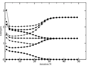
To compute the physical properties of the Kondo model, one diagonalize the Hamiltonians ˜HN iteratively: Knowing the eigenstates |EiN of a chain of length N