Precision bounds for gradient magnetometry with atomic ensembles
Iagoba Apellaniz,1,*Iñigo Urizar-Lanz,1Zoltán Zimborás,1,2,3Philipp Hyllus,1and Géza Tóth1,3,4,†
1Department of Theoretical Physics, University of the Basque Country UPV/EHU, P. O. Box 644, E-48080 Bilbao, Spain
2Dahlem Center for Complex Quantum Systems, Freie Universität Berlin, 14195 Berlin, Germany
3Wigner Research Centre for Physics, Hungarian Academy of Sciences, P.O. Box 49, H-1525 Budapest, Hungary
4IKERBASQUE, Basque Foundation for Science, E-48013 Bilbao, Spain
(Received 7 July 2017; published 8 May 2018)
We study gradient magnetometry with an ensemble of atoms with arbitrary spin. We calculate precision bounds for estimating the gradient of the magnetic field based on the quantum Fisher information. For quantum states that are invariant under homogeneous magnetic fields, we need to measure a single observable to estimate the gradient. On the other hand, for states that are sensitive to homogeneous fields, a simultaneous measurement is needed, as the homogeneous field must also be estimated. We prove that for the cases studied in this paper, such a measurement is feasible. We present a method to calculate precision bounds for gradient estimation with a chain of atoms or with two spatially separated atomic ensembles. We also consider a single atomic ensemble with an arbitrary density profile, where the atoms cannot be addressed individually, and which is a very relevant case for experiments. Our model can take into account even correlations between particle positions. While in most of the discussion we consider an ensemble of localized particles that are classical with respect to their spatial degree of freedom, we also discuss the case of gradient metrology with a single Bose-Einstein condensate.
DOI:10.1103/PhysRevA.97.053603
I. INTRODUCTION
Metrology plays an important role in many areas of physics and engineering [1]. With the development of experimental techniques, it is now possible to realize metrological tasks in physical systems that cannot be described well by classical physics and instead quantum mechanics must be used for their modeling. Quantum metrology [2–5] is the novel field that is concerned with metrology using such quantum mechanical systems.
One of the basic tasks of quantum metrology is magnetom- etry with an ensemble of spin-j particles. Magnetometry with a completely polarized state works as follows. The total spin of the ensemble is rotated by a homogeneous magnetic field perpendicular to it. We would like to estimate the rotation angle or phaseθbased on some measurement; this phase parameter can then be used to obtain the field strength. To determine the rotation angle, one needs, for instance, to measure a spin component perpendicular to the mean spin.
Up to now, it looks as if the total spin behaves like a clock arm and its position tells us the value of θ exactly. At this point, one has to remember that we have an ensemble ofN particles governed by quantum mechanics, and the uncertainty of the spin component perpendicular to the mean spin can never be zero. Hence, simple calculation shows that the scaling of the precision of the phase estimation is (θ)−2∼N, which is called shot-noise scaling [2–5]. However, spin squeezing [6–10] can decrease the uncertainty of one of the components perpendicular to the mean spin and this can be used to increase
*iagoba.apellaniz@gmail.com
†toth@alumni.nd.edu;http://www.gtoth.eu
the precision of the measurements [10]. While it is possible to surpass the shot-noise limit, for the case of a linear Hamiltonian [2–5], no quantum state can have a better scaling in the precision than (θ)−2∼N2, calledHeisenberg scaling.
In recent years, quantum metrology has been applied in many scenarios, from atomic clocks [11–13] and preci- sion magnetometry [14–20] to gravitational wave detectors [21–23]. So far, most of the attention has been paid to the problem of estimating a single parameter. The case of multiparameter estimation for quantum systems is much less studied, possibly, since it can be more complicated due to the noncommutative nature of the problem [24–38].
In this paper, we compute precision bounds for the esti- mation of the magnetic field gradient (see Fig. 1). In gen- eral, in order to achieve these bounds, an estimate of the constant (homogeneous) part of the field is required. Hence, we have to use the formalism of multiparameter estimation.
Magnetometry of this type can be realized with differential interferometry with two particle ensembles, which has raised a lot of attention in quantum metrology [15,39–44]. Another possibility is considering spin chains, which can be relevant in trapped cold ions or optical lattices of cold atoms, where we have individual access to the particles [45–47].
Finally, gradient magnetometry can be carried out using a single atomic cloud, which is very relevant from the point of view of cold gas experiments. One can consider both atomic clouds of localized particles, as well as Bose-Einstein condensates. While most works in magnetometry with a single ensemble focus only on the determination of the strength and direction of the magnetic field, certain measurement schemes for the gradient have already been proposed and tested experimentally. Some schemes use an imaging of the ensemble with a high spatial resolution. They do not count as
FIG. 1. Schematic representation of an atomic ensemble (blue cloud) placed in a magnetic field (green lines) in a Stern-Gerlach apparatus. From the final state the gradient of the field can be estimated. Note that the field intensity changes along the cloud of atoms, while the direction is always the same from north (N) to south (S) within the cloud. For an easier presentation, a setup is shown where the direction of the magnetic field is parallel to the cloud, however, this does not have always to be the case.
single-ensemble methods in the sense we use this expression in our paper since in this case not only collective observables are measured [18–20]. There is a method based on collective measurements of the spin length of a fully polarized ensemble given in Ref. [48]. There is also a scheme based on many-body singlet states described in Ref. [45].
We use the quantum Fisher information (QFI) and the Cramér-Rao (CR) bound in our derivations [4,49–53]. Due to this, our calculations are generally valid for any measurement, thus they are relevant to many recent experiments [14–20,48].
We note that in the case of the spin singlet, our precision bounds are saturated by the metrological scheme presented in Ref. [45].
We can also connect our results to entanglement theory [54–56]. We find that the shot-noise scaling cannot be sur- passed with separable states, while the Heisenberg scaling can be reached with entangled states. However, the shot-noise scaling can be surpassed only if the particle positions are correlated, which is the case, for instance, if the particles attract each other.
Next, we present the main characteristics of our setup.
For simplicity, as well as following recent experiments (e.g., Ref. [18]), we consider an ensemble of spin-jparticles placed in a one-dimensional arrangement. The atoms are then situated along the x axis with y=z=0. We assume that we have particles that behave classically with respect to their spatial state. That is, they cannot be in a superposition of being at two different places. On the other hand, they have internal degrees of freedom, their spin, which is quantum. This is a very good description to many of the cold gas experiments.
Based on these considerations, we assume that the state is factorizable into a spatial part and a spin part as
=(x)⊗(s), (1) where the internal state is decomposed in its eigenbasis as
(s)=
λ
pλ|λλ|. (2) For the spatial part defined in the continuous Hilbert space, we assume that it can be modeled by an incoherent mixture of
pointlike particles as (x)=
P(x)
x|x|xx|dx, (3) where x =(x1,x2, . . . ,xN) is a vector which collects all the particle positions,P(x) is the spatial probability distribution function of the atoms, anddx denotesdx1dx2. . . dxN.Note that the spatial part (3) is diagonal in the position eigen- basis, which simplifies considerably our calculations (see AppendixBfor more details). During the evolution of the state, correlations might arise between the internal and the spatial parts and the product form (1) might not be valid to describe the evolution of the system.
First, we consider spin chains and two particle ensembles at different places. The gradient measurement with two ensem- bles is essentially based on the idea that the gradient is just the difference between two measurements at different locations.
With these systems, it is possible to reach the Heisenberg scaling.
We also examine in detail the case of a single atomic en- semble. Since in such systems the atoms cannot be individually addressed, we assume that the quantum state is permutationally invariant (PI). We show that for states insensitive to the homogeneous magnetic field, one can reduce the problem to a one-parameter estimation scenario. Single-ensemble measure- ments have certain advantages because the spatial resolution can be higher and the experimental requirements are smaller since only a single ensemble must be prepared.
For completeness, we mention the case of Bose-Einstein condensates (BEC). The spatial state in this case is pure
(x)BEC=(||)⊗N, (4) where|is the spatial state of a single particle. Hence, the spatial state is delocalized and it is not an incoherent mixture of various eigenstates ofx. While we do not consider such systems in detail, our formalism could be used to model them.
We now outline the model we use to describe the interaction of the particles with the magnetic field. The field at the atoms is given as
B(x,0,0)=B0+xB1+O(x2), (5) where we neglect the terms of order two or higher, and where O(ξ) is the usual Landau notation to describe the asymptotic behavior of a quantity, in this case for smallξ. We consider the magnetic field pointing in the z direction, hence, B0= B0(0,0,1) and B1=B1(0,0,1). For this configuration, due to the Maxwell equations, with no currents or changing electric fields, we have
divB=0, curlB=(0,0,0). (6) This implies
l=x,y,z∂Bl/∂l=0 and∂Bl/∂m−∂Bm/∂l=0 forl=m.Thus, the spatial derivatives of the field components are not independent of each other. In this paper, however, we consider an elongated trap. In the case of such a quasi-one- dimensional atomic ensemble, only the derivative along the axis of the trap has an influence on the quantum dynamics of the atoms or a double-well experiment.
We determine the precision bounds for the estimation of the magnetic field gradientB1. We calculate how the precision scales with the number of particles. We compare systems
with an increasing particle number, but of the same size.
As discussed later, if we follow a different route, we can obtain results that can incorrectly be interpreted as reaching the Heisenberg limit, or even a super-Heisenberg scaling.
The angular momentum of an individual atom is coupled to the magnetic field, yielding the following interaction term:
h(n)=γ Bz(n)⊗jz(n), (7) where the operatorBz(n)=B0+B1xˆ(n)acts on the spatial part of the Hilbert space and ˆx(n)is the position operator of a single particle. Moreover,jz(n)is a single-particle spin operator, acting on the spin part of the Hilbert space. Finally,γ =gμBwhere gis the gyromagnetic factor andμBcorresponds to the Born magneton, and we set ¯h=1 for simplicity. We use the “ ˆ ” notation to distinguish the operator ˆx from the coordinatex.
Later, we will omit it for simplicity. The Hamiltonian of the entire system is just the sum of all two-particle interactions of the type Eq. (7) and can be written as
H =γ N n=1
Bz(n)⊗jz(n). (8) Equation (8) generates the time evolution of the atomic ensemble.
One could include also the kinetic energy in the Hamilto- nian. Such an extra term causes that the gradient field pushes atoms in state|0into one direction, while atoms in state|1 into the other direction. In our work, we do not take into account this effect. Moreover, we do not include in the model the initial thermal dynamics of the particles. Both of these effects are negligible in a usual setup, as shown in AppendixA.
We calculate lower bounds on the precision of estimatingB1 based on a measurement on the state after it passed through the unitary dynamicsU =exp(−iH t), wheret is the time spent by the system under the influence of the magnetic field. The unitary operator can be rewritten as
U =e−i(b0H0+b1H1), (9) where thebi =γ Bit. The generator describing the effect of the homogeneous field is given as
H0= N n=1
jz(n)=Jz, (10) while the generator describing the effect of the gradient is
H1= N n=1
x(n)jz(n). (11) We omit⊗and the superscripts (x) and (s) for simplicity, and use them only if it is necessary to avoid confusions.
The operatorsH0 andH1commute with each other. How- ever, it is not necessarily true that the operators we have to measure to estimateb0orb1can be simultaneously measured.
The reason for that is that both operators to be measured act on the same atomic ensemble. If the measurement operators do not commute with each other, then the precision bound obtained from the theory of QFI cannot necessarily be reached. For the particular cases studied in this paper, we prove that a simulta- neous measurement to estimate both the homogeneous and the
gradient parameter can be carried out (see AppendixE). On the other hand, in schemes in which the gradient is calculated based on measurements on two separate atomic ensembles or different atoms in a chain, the measuring operators can always commute with each other [14,15,46].
The paper is organized as follows. In Sec. II, general precision bounds for the estimation of the gradient of the magnetic field are presented. In Sec.III, we compute precision bounds for relevant spatial configurations appearing in cold atom physics such as spin chains and two ensembles spatially separated from each other. In Sec. IV, we consider a single atomic ensemble in a PI state and we calculate the precision bounds for various quantum states, such as the singlet spin state or the totally polarized state. In Sec. V, we consider Bose-Einstein condensates.
II. PRECISION BOUNDS FOR ESTIMATING THE GRADIENT
In this section, we show how the QFI helps us to obtain the bound on the precision of the gradient estimation. First, we discuss gradient magnetometry using quantum states that are insensitive to homogeneous fields. In this case, we need to estimate only the gradient and do not have to know the homogeneous field. Hence, this case corresponds to a single- parameter estimation problem.
Then, we discuss the case of quantum states sensitive to homogeneous fields. Even in this case, we are interested only in the gradient, and we do not aim at estimating the homogeneous field. In spite of this, gradient estimation with such states is a two-parameter estimation task. We introduce the basics of multiparameter quantum metrology, and we adapt that formalism to our problem. We also show that the precision bound obtained does not change under spatial translation, which will be used later to simplify our calculations. In AppendixE, we show that even the precision bounds for states sensitive to the homogeneous field, appearing in this paper, are saturable.
Next, we summarize important properties of the QFI used throughout this paper (for reviews, see Refs. [2,4,53,57–62]).
Let us consider a quantum state with the eigendecomposition
=
k
pk|kk|. (12) For two arbitrary operatorsAandB,and a state[Eq. (12)], the QFI is defined as [4,49–51,53]
FQ[,A,B] :=2
k,k
(pk−pk)2
pk+pk Ak,kBk,k, (13) whereAk,k = k|A|kandBk,k= k|B|k. If the two oper- ators are the same then, from Eq. (13), the usual form of the QFI is obtained:
FQ[,A]≡FQ[,A,A]=2
k,k
(pk−pk)2 pk+pk
|Ak,k|2. (14)
We list some useful properties of the QFI:
(i) Based on Eq. (13),FQ[,A,B] is linear in the second and third arguments
FQ
,
i
Ai,
j
Bj
=
i,j
FQ[,Ai,Bj]. (15) This will make it possible to calculate the QFI for collective quantities based on the QFI for single-particle observables.
(ii) The QFI remains invariant if we exchange the second and the third arguments
FQ[,A,B]=FQ[,B,A]. (16) Equation (16) will help to simplify our calculations.
(iii) The following alternative form, FQ[,A,B]=4AB −8
k,k
pkpk
pk+pk
Ak,kBk,k, (17) is also useful since the correlation appears explicitly.
(iv) For pure states, Eq. (13) simplifies to
FQ[|ψ,A,B]=4(ABψ − AψBψ). (18) Using Eq. (18) forA=B,we obtain that for pure states the QFI equals four times the variance, i.e.,FQ[|ψ,A]=4(A)2. (v) The QFI is convex on the space of the density matrices, i.e.,
FQ[p1+(1−p)2,A]pFQ[1,A]+(1−p)FQ[2,A], (19) Hence, when maximizing the QFI, we need to carry out an optimization over pure states only.
In the following, we show the general form of the expres- sions giving the precision bounds for states insensitive to the homogeneous field, as well as for states sensitive to it. We also show that both bounds are invariant under the spatial translation of the system which makes the computing for particular cases much easier.
A. Precision bound for states insensitive to homogeneous fields:
Single-parameter dependence
We will now consider quantum states that are insensitive to the homogeneous field. For such states,
[,H0]=0 (20)
holds. Hence, the unitary time evolution given in Eq. (9) is simplified to
U=e−ib1H1, (21) and the evolved state is a function of a single unknown parameterb1.
When estimating a single parameter, the Cramér-Rao bound gives the best achievable precision as [4]
(b1)−2|max=FQ[,H1]. (22) It is always possible to find a measurement that saturates the precision bound (22), which is indicated using the notation
“|max=”.
Observation 1. For states insensitive to the homogeneous fields, the maximal precision of the estimation of the gradient parameterb1is given as
(b1)−2|max= N
n,m
xnxmP(x)dxFQ
(s),jz(n),jz(m) , (23) where the integral represents the correlation between the particle positionsxn andxm. Moreover, Eq. (23) is transla- tionally invariant, i.e., it remains the same after an arbitrary displacementdof the form of
Ud =exp(−idPx), (24) where d is the distance displaced and Px is the sum of all single-body momentum operatorsp(n)x in thexdirection.
Proof.We have to evaluate the right-hand side of Eq. (22).
The state is a tensor product of the spatial and internal parts, and the spatial part is an incoherent mixture of position eigenstates, as in Eqs. (1) and (3). Hence, the eigenstates are|x,λ, where
|x and |λ are defined in the spatial and internal Hilbert spaces, respectively. Then, the matrix elements ofH1, which is diagonal in the spatial subspace, are obtained as
(H1)x,λ;y,ν =δ(x−y)λ| N n=1
xnj(n)|ν. (25) Calculating Eq. (14) forA=H1, Eq. (22) leads to Eq. (23) (see AppendixCfor details).
In the last part of the proof, we show that the precision (23) remains the same for any displacement of the system.
We use the Heisenberg picture in which the operators must be transformed instead of the states. After the displacement, the operatorH1describing the effect of the gradient is obtained as H1(d)=H1−dH0. (26) Hence, the unitary evolution operator of the displaced system is obtained as
U(d)=e−i[b0H0+b1H1(d)]=e−i[(b0−b1d)H0+b1H1]. (27) Using the commutation relation (20), we can see that Eq. (27) is equal to the time evolution given in Eq. (21).
B. Precision bound for states sensitive to homogeneous fields:
Two-parameter dependence
We now show how to obtain the precision bounds for states sensitive to the homogeneous field. The homogeneous field rotates all the spins in the same way, while the field gradient rotates the spins differently depending on the position of the particles. Hence, in order to estimateb1,we have to consider the effect of a second unknown parameterb0. Note, however, that we are not interested to estimateb0precisely, we just need it to estimateb1.
In this case, the metrological performance of the quantum state is given by the 2×2 Cramér-Rao matrix inequality [4]
CF−1Q , (28)
where the covariance matrix is defined as Cij = bibj − bibj. The matrix elements of the quantum Fisher
information matrixFQare
Fij :=FQ[,Hi,Hj]. (29) Unlike in the case of single-parameter estimation, Eq. (28) can be saturated only if the measurements for estimating the two parameters are compatible with each other [4,51,63]. Hence, we use “” instead of “|max” for the bounds for quantum states sensitive to the homogeneous fields.
Using the well-known formula for the inverse of 2×2 matrices, Eq. (28) yields
(b1)−2 F11−F01F10
F00
(30) for the precision ofb1.
Observation 2. For states sensitive to the homogeneous field, the expression to compute the precision bound for the gradient parameter takes the following form:
(b1)−2 N
n,m
xnxmP(x)dxFQ
(s),jz(n),jz(m)
−
N n=1
xnP(x)dxFQ
(s),jz(n),Jz
2 FQ[(s),Jz] . (31) Moreover, the bound (31), similarly to Eq. (23), is invariant under spatial translations of the system.
Proof. To obtain the bound (31), we need to consider the matrix elements of QFI one by one. First of all, we compute F11which has the same form as Eq. (23):
F11= N
n,m
xnxmP(x)dxFQ
(s),jz(n),jz(m)
. (32) Next, we have thatH0, similarly to Eq. (25), is diagonal in the spatial|xbasis, and its matrix elements in the|x,λbasis of the state are written as
(H0)x,λ;y,ν =δ(x−y)λ| N n=1
jz(n)|ν. (33) With this we obtainFQ[,H0,H0] as
F00=FQ[(s),Jz]. (34) Note that Eq. (34) is not a function of the whole state but only of the internal(s) state. Finally, we compute F01 and F10. SinceF01=F10, we have to compute only one of them. Using Eqs. (33) and (25),FQ[,H0,H1] is obtained as
F01= N n=1
xnP(x)dxFQ
(s),jz(n),Jz
. (35) With these results, Eq. (31) follows (see AppendixC).
Let us now determine the bound on the precision for estimating the gradient on the translated system. We have to compute first the QFI matrix elements. We use the linearity of the last two arguments ofFQ[,A,B] given in Eq. (15), the fact thatH0remains unchanged in the Heisenberg picture. We also use the formula (26) for the shiftedH1operator. The diagonal element of the QFI matrix corresponding to the measurement
of the homogeneous field is
F00(d)=FQ[,H0(d)]=F00, (36) hence, it does not change due to the translation. For the diagonal element corresponding to the gradient measurement we obtain F11(d)=F11−2dF01+d2F00. (37) Finally, for the off-diagonal element, we get
F01(d)=F01−dF00. (38) After determining all the elements of the QFI matrix, the bound for a displaced system can be obtained as
(b1)−2F11(d)−[F01(d)]2 F00(d)
=F11−2dF01+d2F00
−F012 −2dF01F00+d2F002 F00
. (39) The bound in Eq. (30) can be obtained from the right-hand side of Eq. (39) with straightforward algebra.
III. SPIN CHAIN AND TWO SEPARATED ENSEMBLES FOR MAGNETOMETRY
After presenting our tools in Sec.II, we start with simple examples to show how our method works. We calculate precision bounds for gradient metrology for spin chain and for two-particle ensembles separated by a distance.
Before considering the setups mentioned above, we intro- duce various quantities describing the distribution of the par- ticles based on the probability distribution function appearing in Eq. (3). The mean particle position is
μ=
N n=1xn
N P(x)dx. (40) The standard deviation of the particle positions, describing the size of the system, is computed as
σ2=
N n=1x2n
N P(x)dx−μ2. (41) Finally, the covariance averaged over all particle pairs is
η=
N n=mxnxm
N(N−1) P(x)dx−μ2. (42) The covariance is a large positive value if the particles tend to be close to each other, while it is negative if they tend to avoid each other.
After presenting the fundamental quantities above, let us study concrete metrological setups. The first spatial state we consider is given byNparticles placed equidistantly from each other in a one-dimensional spin chain, as shown in Fig. 2.
Such a system has been studied also in the context of a single- parameter estimation in the presence of collective phase noise [44]. The probability density function describing such a system is
P(x)= N n=1
δ(xn−na), (43)
FIG. 2. A one-dimensional chain of six spin-jatoms (blue disks) confined in a potential (gray area). (a) The ensemble is initially totally polarized along theydirection. The magnetic fieldBzpoints outward from the figure. The spin chain is along thexdirection. (b) If the magnetic field has a nonzero gradient, then it affects the spins of the individual atoms differently depending on the position of the atoms.
whereais the distance between the particles in the chain. For this system, the average position of thenth particle is
xnP(x)dx=na, (44) whereas the two-point average (42) is
xnxmP(x)dx=nma2. (45) The standard deviation defined in Eq. (41) is obtained as
σch2 =a2N2−1
12 . (46)
Next, we will obtain precision bounds for particles placed in a spin chain.
Observation 3. Let us consider a chain ofNspin-jparticles placed along thexdirection separated by a constant distance, and a magnetic field pointing in thezdirection. Then, for the spin-state totally polarized in theydirection,
|ψtp = |j⊗yN, (47) the precision bound is given by
(b1)−2|max=2σch2Nj. (48) Here,σchdenotes the standard deviation of the average position of the particles for the chain (ch).
Proof. We use the precisions bound for states sensitive to the homogeneous field given in Eq. (31). We obtain
(b1)−2|max= N
n,m
nma2FQ
|j⊗yN,jz(n),jz(m)
−
N n=1anFQ
|j⊗yN,jz(n),Jz2
FQ
|j⊗yN,Jz,Jz
=2a2N2−1
12 Nj. (49)
Note that the bound can be saturated (see AppendixE). Here, for the last equality we used the definitions of the average quantites given in Eqs. (44) and (45) and we also used Eq. (18) giving the QFI for pure states. We can see that the standard
deviation given in Eq. (46) coincides with a factor we have in Eq. (49), with which we conclude the proof.
Note that the bound (49) seems to scale with the third power of the particle numberN, and hence seems to overcome the ultimate Heisenberg limit. The reason is that the length of the chain increases as we introduce more particles into the system.
We should compare the metrological usefulness of systems with different particle numbers, but of the same size. In our case, we use throughout the paper the standard deviation of the averaged particle positions as a measure of the spatial size of the system, and normalize the results with it. One can miss this important point since when only the homogeneous field is measured such a normalization is not needed.1
After the spin chain, we consider estimating the gradient with two ensembles of spin-j atoms spatially separated from each other. Such systems have been realized in cold gases (e.g., Ref. [64]), and can be used for differential interferometry [15,39,44]. We will determine the internal state with the maximal QFI.
Let us assume that half of the particles are at one position and the rest at another one, both places at a distanceafrom the origin. The probability density function of the spatial part is
P(x)=
N/2
n=1
δ(xn+a) N n=N/2+1
δ(xn−a). (50) Such a distribution of particles could be realized in a double- well trap, where the width of the wells is negligible compared to the distance between the wells. To distinguish the two wells we use the labels “L” and “R” for the left-hand side and right- hand side wells, respectively. Based on these, we obtain the single-point averages as
xnP(x)dx=
−a ifn∈L,
+a ifn∈R. (51) The two-point correlation functions are
xnxmP(x)dx=
+a2 if (n,m)∈(L,L) or (R,R),
−a2 if (n,m)∈(L,R) or (L,R). (52) For the average particle position we obtainμ=0,while the standard deviation for the spatial state in the double well (dw) is
σdw2 =a2. (53) Next, we calculate the achievable precision of the gradient estimation.
Observation 4. For the case of two ensemble ofN spin-j particles, the state that maximizes the QFI is
|ψ=|j . . . j(L)|−j . . .−j(R)√+|−j . . .−j(L)|j . . . j(R)
2 .
(54)
1This comment is relevant for the setup of Ref. [46], where the precision of the gradient estimation seems to reach the Heisenberg scaling. In reality, the shot-noise scaling has not been overcome. The question of normalization is also important for the setup in Ref. [47].
The best achievable precision is given as
(b1)−2|max=4σdw2 N2j2. (55) Equation (55) agrees with the results obtained in Ref. [39].
Proof. The state given in Eq. (54) is insensitive to the homogeneous field, hence, we have to use the formula (23) to bound the precision. We obtain
(b1)−2|max=
(n,m)=
(L,L),(R,R)
a2FQ
|ψ,jz(n),jz(m)
+
(n,m)=
(L,R),(R,L)
−a2FQ
|ψ,jz(n),jz(m) . (56)
For the state (54), the equation above, (56), yields (b1)−2|max =
(n,m)=
(L,L),(R,R)
a2j2+
(n,m)=
(L,R),(R,L)
−a2(−j2)
=4a2N2j2, (57) where we have used the definition of the QFI for pure states given in Eq. (18). A factor in Eq. (57) can be identified with the standard deviation (46) from which the proof follows.
It is interesting to simplify the QFI for product states states
|ψ(L)⊗ |ψ(R), where|ψ(L)and|ψ(R)are pure states ofN/2 particles each. This approach is also discussed in Ref. [39].
Such states can reach the Heisenberg limit, while they are easier to realize experimentally than states in which the particles in the wells are entangled with each other.
Before obtaining the precision for the case above, we present a method to simplify our calculations. The system is at the origin of the coordinate system such that for mean particle position given in Eq. (40),
μ= nxn
N P(x)dx =0 (58) holds. Thus, the second term in the expression for the bound for states sensitive to the homogeneous field (31) is zero since allFQ[(s),jz(n),Jz] are equal considering product states of two equal permutationally invariant states|ψ(L)⊗ |ψ(R). Hence, the bounds for states insensitive and sensitive to the homogeneous field, Eqs. (23) and (31), respectively, are the same in this case.
We now computeFQ[ρ,H1] for the case when the state is sensitive to the homogeneous field, hence, we use the bound on the precision given in Eq. (31). Using the the probability density distribution function given in Eq. (50), and following steps leading to Eq. (57), we obtain
FQ[|ψ(L)|ψ(R),H1]=2a2FQ
|ψ(L),Jz(L)
, (59) where we used thatFQ[|ψ(L),Jz(L)]=FQ[|ψ(R),Jz(R)]. Note that our results concerning using product states for magnetom- etry can be interpreted as follows. In this case, essentially the homogeneous field is estimated in each of the two wells, and then the gradient is computed from the measurement results.
The bounds for these type of states are also saturable (see AppendixE).
We will now present precision bounds for various well- known quantum states in the two wells. We consider the
TABLE I. Precision for differential magnetometry for various product states of the type |ψ(L)⊗ |ψ(R) in the two ensembles.
Note that there are NL=NR=N/2 particles in each ensemble.
In the second column, we show the QFI for the estimation of the homogeneous field appearing in the literature, for states with NL
particles. The third column shows the result for the bounds obtained with Eq. (59).
|ψ FQ[|ψ,Jz] (b1)−2|max
|j⊗yNL 2NLj 2a2Nj
|ψsep 4NLj2 4a2Nj2
|GHZ NL2 a2N2/2
|DNLx NL(NL+2)/2 a2N(N+4)/4
Greenberger-Horne-Zeilinger (GHZ) state [65–70]
|GHZ = |00. . .00 + |11√ . . .11
2 , (60)
where|0and|1are the eigenstates ofjz(n) with eigenvalues
−12and+12,respectively. We also consider unpolarized Dicke states [71–78]
|DNl = N
N/2
−1/2
k
Pk |0⊗lN/2⊗ |1⊗lN/2
, (61)
where l=x,y,zand the summation is over all Pk permuta- tions. Such states are the symmetric superposition of product states with an equal number of|0l’s and|1’s. Based on these, in TableIwe summarized the precision bounds for states of the type|ψ(L)⊗ |ψ(R)for the double-well case.
IV. MAGNETOMETRY WITH A SINGLE ATOMIC ENSEMBLE
In this section, we discuss magnetometry with a single atomic ensemble. We consider a one-dimensional ensemble of spin-j atoms placed in a trap which is elongated in the x direction. The setup is depicted in Fig.3. In the second part of the section, we calculate precision bounds for the gradient estimation with some important multiparticle quantum states, for instance, Dicke states, singlet states, and GHZ states.
A. Precision bound for an atomic ensemble
In an atomic ensemble of many atoms, typically the atoms cannot be individually addressed. We will take this into account by considering states for which both the internal state(s)and the probability distribution functionP(x), appearing in Eq. (3),
FIG. 3. An ensemble of spin-j atoms in a cigar-shaped trap elongated in thexdirection. The magnetic field, represented by green arrows, points in thezdirection and it is linear inx. Its strength is proportional to the density of the field lines.
FIG. 4. Possible particle distributions for a chain of atoms on a 1D lattice, assuming that Eq. (62) holds for the probability distribution function. We consider three cases, determined by the value of the covarianceη. (Top) The atoms bunch together due to high correlation in the positions. As explained in the text, this leads to the possibility of estimating well the magnetic field at each point, and hence possibly obtaining a very good estimate of the gradient parameter. (Middle) Due to the small covariance the particles fill up the sites more uniformly. (Bottom) The negative correlation makes the particles be far from each other, filling the trap uniformly.
are PI. The permutational invariance ofP(x) implies that P(x)= 1
N!
k
Pk[P(x)] (62) holds, where the summation is over all possible permutations Pkof the variablesxn. Hence, we do not need to sum over all possiblen’s in Eqs. (40) and (41), and neither to sum over alln’s andm’s in Eq. (42). All the terms in each sum are equal to each other due to the permutationally invariance of the probability distribution function (62).
An interesting property of the covariance (42) is that it can only take values bounded by the variance in the following way:
−σ2
N−1 ησ2, (63) where both the lower and the upper bounds are proportional to the varianceσ2.See Fig.4for examples on how different correlations are obtained in an atomic 1D lattice.
Next, we present precision bounds for PI states.
Observation 5. The maximal precision achievable by a single atomic ensemble insensitive to homogeneous fields is
(b1)−2|max =(σ2−η) N n=1
FQ
(s),jz(n)
. (64) The precision given in Eq. (64) can be reached by an op- timal measurement. Nevertheless, it is worth to note that the precision cannot surpass the shot-noise scaling because FQ[(s),jz(n)] cannot be larger thanj2.Moreover,ηcannot be smaller than−σ2/(N−1) due to Eq. (63), which makes its contribution negligible for largeN.
Proof.From the definition of the QFI for states insensitive to the homogeneous field [Eq. (23)], we obtain the bound for
a single ensemble as (b1)−2|max =
N n,m
xnxmP(x)dxFQ
(s),jz(n),jz(m)
= N n=1
σ2FQ
,jz(n) +
N n=m
ηFQ
,jz(n),jz(m) .
(65) Then, we have to use the fact that for states insensitive to the homogeneous fieldsFQ[,Jz]=0 holds, which implies
FQ[,Jz]= N
n,m
FQ
,jz(n),jz(m)
=0. (66)
Based on this, for such states the sum of QFI terms involving two operators can be expressed with the sum of QFI terms involving a single operator as
N n=m
FQ
,jz(n),jz(m)
= − N n=1
FQ
,jz(n)
. (67) Substituting Eq. (67) into Eq. (65), Observation5follows.
Observation 6. For states sensitive to homogeneous fields, the precision of estimating the gradient is bounded from above as
(b1)−2|max=(σ2−η) N n=1
FQ
(s),jz(n)
+ηFQ[(s),Jz], (68) which may surpass the shot-noise scaling whenever η is a positive constant.
Proof.We start from Eq. (31) and take into account that in this case the bound is saturable (see AppendixE). As explained in Sec.II B, if we move the system, the precision bounds do not change. We then move our system to the origin of the coordinate system yieldingμ=0,and making the second term appearing in Eq. (31) zero. Thus, we only compute the first term in Eq. (31) and obtain
(b1)−2|max = N n=1
σ2FQ
,jz(n) +
N n=m
ηFQ
,jz(n),jz(m) .
(69) Then, we addηN
n=1FQ[,jz(n)] to the last term and subtract it from the first term to make the expression more similar to
Eq. (64).
Note that the second term on the right-hand side of Eq. (68) is new in the sense that it did not appear in the bound for states insensitive to homogeneous fields given in Eq. (64). Even if the first term cannot overcome the shot-noise limit, in the second term the covariance is multiplied by the QFI for estimating the homogeneous field and therefore this concrete term, for extremely correlated particle positions, allows to achieve the Heisenberg scaling.
B. Precision limit for various spin states
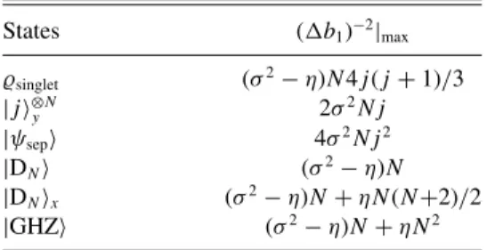
In this section, we present the precision limits for various classes of important quantum states such as the totally polar- ized state, the state having the best precision among separable states, the singlet state, the Dicke state (61), or the GHZ state (60). We calculate the precision bounds presented before, (64) and (68), for these systems.
1. Singlet states
A pure singlet state is a simultaneous eigenstate of the collectiveJzandJ2operators, with an eigenvalue zero for both operators. We will now consider PI singlet states. Surprisingly, the precision bound is the same for any such state. PI singlet states are very relevant for experiments since they have been experimentally created in cold gases [79,80] while they also appear in condensed matter physics [81].
Let us now see the most important properties of singlet states of anN-particle system. There are several singlets pairwise orthogonal to each other. The number of such singlets, D0, depends on the particle spinj and the number of particlesN. It is the most natural to write the singlet state in the angular momentum basis. The basis states are|J,Mz,D,which are the eigenstates ofJx2+Jy2+Jz2with an eigenvalueJ,and of Jzwith an eigenvalueMz.The labelDis used to distinguish different eigenstates corresponding to the same eigenvalue of JandJz. Then, a singlet state can be written as
(s)singlet=
D0
D=1
pD|0,0,D0,0,D|, (70) where
DpD=1.
Let us see some relevant single-particle expectation values for the singlet. Due to the rotational invariance of the singlet (s)singlet, we obtain that
jx(n)2
= jy(n)2
= jz(n)2
(71) holds. We also know that for the sum of the second moments of the single-particle angular momentum components
jx(n)2
+ jy(n)2
+ jz(n)2
=j(j +1) (72) holds. Hence, the expectation value of the second moment of the single-particle angular momentum component is obtained as
jz(n)2
=j(j +1)
3 . (73)
After discussing the main properties of the singlet states, we can now obtain a precision bound for gradient metrology with such states.
Observation 7. For PI spin states living in the singlet subspace, i.e., states composed of vectors that have zero eigenvalues for Jz and J2 and all their possible statistical mixtures, the precision of the magnetic gradient parameter is bounded from above as
(b1)−2singlet|max=(σ2−η)N4j(j+1)
3 . (74)
Proof.First compute the QFI for the one-particle operator jz(n),FQ[(s),jz(n)].For that we need that whenjz(n) acts on a
singlet state, produces a state outside of the singlet subspace.
Hence,
0,0,D|jz(n)|0,0,D =0 (75) for any pair of pure singlet states. Then, we use the formula (17) to compute the QFI. The second term of Eq. (17) is obtained as
8
D,D
pDpD
pD+pD
0,0,D|jz(n)|0,0,D2=0, (76) due to Eq. (75). It follows that the single-particle QFI for any singlet equals four times the second moment of the angular momentum component
FQ
(s)singlet,jz(n)
=4 tr
(s)singlet jz(n)2
. (77) Note that Eq. (77) is true even though(s)singletis a mixed state.
Inserting the expectation value of the second moment of the angular momentum component given in Eq. (73) into Eq. (77), we obtain FQ[(s)singlet,jz(n)] for any n.Then, we have all the ingredients to evaluate the maximal precision given in Eq. (64), and with that we prove the Observation.
As mentioned earlier, singlet states are insensitive to homo- geneous magnetic fields, hence determining the gradient leads to a single-parameter estimation problem. This implies that there is an optimal operator that saturates the precision bound given by Eq. (74). However, it is usually very hard to find this optimal measurement, although a formal procedure for this exists [4]. In Ref. [45], a particular setup for determining the magnetic gradient with PI singlet states was suggested by the measurement of theJx2 collective operator. For this scenario the precision is given by
(b1)−2= ∂b1
Jx22
Jx22 . (78) In Appendix D, we show that this measurement provides an optimal precision for gradient metrology for all PI singlets.
2. Totally polarized state
The totally polarized state can easily be prepared experi- mentally. It has already been used for gradient magnetometry with a single atomic ensemble [18,19]. For the gradient measurement as for the measurement of the homogeneous field, the polarization must be perpendicular to the field we want to measure.
We chose as before the totally polarized state alongyaxis, given in Eq. (47). The relevant variances for the state (47) are (Jz)2tp =Nj/2, (79a) jz(n)2
tp =j/2 (79b)
for all n. Based on Eq. (18), for pure states the QFI is just four times the variance. Hence, from Eq. (79b), we obtain FQ[,jz(n)]=2j and FQ[,Jz]=2Nj. Then, the bound on the sensitivity can be obtained from the formula for PI states sensitive to homogeneous fields (68) as
(b1)−2tp |max=2σ2Nj. (80)