Entanglement negativity bounds for fermionic Gaussian states
Jens Eisert,1Viktor Eisler,2,3and Zoltán Zimborás1,4
1Dahlem Center for Complex Quantum Systems, Freie Universität Berlin, 14195 Berlin, Germany
2Institute of Theoretical and Computational Physics, Graz University of Technology, Petersgasse 16, 8010 Graz, Austria
3MTA-ELTE Theoretical Physics Research Group, Eötvös Loránd University, Pázmány Péter sétány 1/a, 1117 Budapest, Hungary
4Department of Theoretical Physics, Wigner Research Centre for Physics, Hungarian Academy of Sciences, H-1525 Budapest P.O. Box 49, Hungary
(Received 24 February 2018; published 13 April 2018)
The entanglement negativity is a versatile measure of entanglement that has numerous applications in quantum information and in condensed matter theory. It can not only efficiently be computed in the Hilbert space dimension, but for noninteracting bosonic systems, one can compute the negativity efficiently in the number of modes.
However, such an efficient computation does not carry over to the fermionic realm, the ultimate reason for this being that the partial transpose of a fermionic Gaussian state is no longer Gaussian. To provide a remedy for this state of affairs, in this work, we introduce efficiently computable and rigorous upper and lower bounds to the negativity, making use of techniques of semidefinite programming, building upon the Lagrangian formulation of fermionic linear optics, and exploiting suitable products of Gaussian operators. We discuss examples in quantum many-body theory and hint at applications in the study of topological properties at finite temperature.
DOI:10.1103/PhysRevB.97.165123
I. INTRODUCTION
Entanglement is the distinct feature that makes quantum mechanics fundamentally different from a classical statisti- cal theory. Undeniably playing a pivotal role in quantum information theory, in notions of key distribution, quantum computing and simulation, it is becoming clear that notions of entanglement have the potential to add a fresh perspective to the study of systems of condensed matter physics. Notions of entanglement entropies and spectra are increasingly used to capture properties of quantum systems with many degrees of freedom [1–3]. The entanglement entropy based on the von- Neumann entropy plays here presumably the most important role [1,2]. However, it makes sense as an entanglement measure only for pure states. Hence, early on, computable measures of entanglement such as the entanglement negativity [4–7]
have been considered in the context of the study of quantum many-body systems. In fact, one of the earliest studies on entanglement properties of ground states of local Hamiltonians considered this entanglement measure [8], which was followed by a series of works on harmonic lattices [9–14].
Recent years have seen a revival of interest in studies of entanglement negativity, and the problem has been attacked using a number of different approaches. Numerical studies were performed for various spin chains via tensor network cal- culations [15–18], Monte Carlo simulations where the replica trick comes into play [19,20], or via numerical linked cluster expansion [21]. On the analytical side, major developments include the conformal field theory (CFT) approach [22,23], which has also been extended to finite temperature [24,25], nonequilibrium [24,26–28], and off-critical [29] scenarios.
For some particular spin chains, there are even exact results available [30–33]. Studies of negativity have also been carried
out for two-dimensional lattices [34,35] with a particular emphasis on topologically ordered phases [36–39].
The entanglement negativity—first proposed in Ref. [4], elaborated upon in Ref. [40], and proven to be an entanglement monotone in Refs. [5,6]—can be computed efficiently in the Hilbert space dimension for spin systems. For Gaussian bosonic systems, as they occur as ground and thermal states of noninteracting models, the negativity can even be efficiently computed in the number of modes [6,8,41,42]. This is possible because the partial transpose [43] on which the entanglement negativity is based, reflects partial time reversal [44], which maps bosonic Gaussian states to Gaussian operators. This is in sharp contrast to the situation for fermionic Gaussian systems, where the partial transpose is, in general, no longer a fermionic Gaussian operator [45]. Consequently, there is still no efficiently calculable formula known for the nega- tivity. This is unfortunate, since Gaussian (or free) fermionic systems are specifically rich. For example, some well-known models showing features of topological properties such as Kitaev’s honeycomb lattice model are noninteracting [46].
Also, one of the most paradigmatic one-dimensional models exhibiting edge states in a topologically nontrivial phase, the Su-Schrieffer-Heeger (SSH) model [47] is a noninteracting (or quasifree) fermionic system.
The lack of a formula for negativity of fermionic Gaus- sian states has stimulated a concerted research activity on identifying good bounds [45,48]. In this work, we make a fresh attempt at proving tight bounds to the entanglement negativity. Each bound considered here depends exclusively on the covariance matrix of the Gaussian state at hand, and thus is efficiently computable in the number of modes. In particular, the lower bound makes use of a pinching transformation of the covariance matrix, while the first of two upper bounds requires
techniques of semidefinite programming. The second upper bound was already proposed in a CFT context [48], which is now elaborated and closed form expressions for arbitrary fermionic Gaussian states are given. We also test our bounds by estimating the negativity between adjacent segments in the SSH model and the XX chain, both in the ground state and at finite temperatures.
The paper is structured as follows. In Sec.II, we introduce the notation used in the rest of this work and define the negativity, followed by some basic examples given in Sec.III.
The lower bound is constructed in Sec.IV, whereas Secs.V and VI deal with two different upper bounds, based on semidefinite programming and products of Gaussian operators, respectively. Numerical checks of the bounds are presented in Sec.VII, followed by our concluding remarks in Sec.VIII.
II. PRELIMINARIES A. Fermionic quantum systems
Throughout this work, we consider quantum systems con- sisting of a set of fermionic modes; the annihilation and cre- ation operators{f1,f1†, . . . fk,fk†}associated with the modes generates the CAR algebra, i.e., the algebra of operators respecting the canonical anticommutation relations. In many contexts, it is convenient to refer rather to Majorana fermions than to the original ones, by defining
m2j−1 =fj†+fj, m2j =i(fj†−fj) (1) forj =1, . . . ,k. Given a stateρ, the second moments of the Majorana fermions can be collected in the covariance matrix γ ∈R2k×2k, with entries
γj,l = i
2tr(ρ[mj,ml]). (2) It is easy to see that this matrix satisfies
γ = −γT, iγ 1. (3) We will denote the set of such covariance matrices ofkmodes asCk⊂R2k×2k.
A fermionic Gaussian stateρis completely defined by its covariance matrix, as one can express the expectation value of any Majorana monomial through the Wick expansion
tr(ρ mj1mj2. . . mj2p)=(−i)p
π
sgn(π) p l=1
γjπ(2l−1),jπ(2l), (4) where the indices of the Majorana operators are different and the sum runs over all pairingsπ[with sgn(π) denoting the sign of the pairing].
Considering a Gaussian (or quasifree, as it is also called) unitary
V=e−14j,lKj,lmjml (5) (whereK∈R2k×2kwithK= −KT) and a Gaussian stateρ, the evolved stateρ=Vρ V†remains Gaussian. On the level of the covariance matrices, this mapping can be represented by the transformation
γ →OKγ OKT, (6)
whereOK =e−K ∈SO(2k). In this context, a commonly used tool is that a covariance matrix can be brought to a normal form by means of such a special orthogonal mode transformationO,
Oγ OT = k
j=1
xj
0 −1
1 0
, (7)
withxj ∈[−1,1] corresponding to the presence or absence of a fermion in the normal mode decomposition.
A Gaussian state is called particle-number conserving if it commutes with the particle-number operator k
j=1fj†fj. In this case, the expectation values of the pairing opera- tors vanish, i.e., fjfl = fj†fl† =0. Thus the 2k×2k covariance matrix γ can be completely recovered from the k×kcorrelation matrixCj,l = fj†fl. Moreover, such a state remains particle-number conserving and Gaussian under a mode transformations of the form e−ij,lRj,lfj†fl (where R is a Hermitian matrix), and the corresponding map on the correlation matrix level, analog of Eq. (6), is given by
C→URC UR†, (8) whereUR =e−iR∈U(k).
B. Partial transpose and negativity
Let us now turn to the definition of entanglement negativity.
Consider a bipartite fermionic system composed of two subsys- temsAandBcorresponding to Majorana modes{m1, . . . m2n} and{m2n+1, . . . m2k}, respectively. Following the literature, we will refer to such a setup as a bipartite system ofn×(k−n) modes. Given a bipartite fermionic stateρ, the entanglement negativity is defined as
N =1
2( ρTB 1−1), (9)
where . 1is the trace norm and the superscriptTBdenotes par- tial transposition with respect to subsystemB. The logarithmic negativity as a derived quantity is
E =ln ρTB 1. (10) Both quantities have their significance, and the latter is an entanglement monotone despite not being convex [7], as well as an upper bound to the distillable entanglement. Since at the heart of the problem under consideration here is the assessment of ρTB 1, a bound to the latter gives immediately a bound to both the negativity and the logarithmic negativity.
To proceed, we first need to represent the action of the partial transposition on the density operator. Using the notations m0j =1andm1j =mj, a fermionic state can be written as
ρ=
τ
wτmτ11. . . mτ2k2k, (11) where the summation runs over all bit-strings τ = (τ1, . . . ,τ2k)∈ {0,1}×2kof length 2k.1The partial transpose of
1Note that a physical fermionic state must also commute with the parity operatorP = 2kj=1mj, i.e., one haswτ =0 when2k
j=1τjis odd.
ρwith respect to subsystemBis the transformation that leaves theAMajorana modes invariant and acts as a transpositionR on the operators built up from modes ofB, i.e.,
ρTB =
τ
wτmτ11. . . mτ2n2nR
mτ2n2n+1+1. . . mτ2k2k
. (12) As shown in Ref. [45], the action ofRin a suitable basis can be written as
R
mτ2n2n+1+1. . . mτ2k2k
=(−1)f(τ)mτ2n2n+1+1. . . mτ2k2k, (13) where
f(τ)=
0 if2k
j=2n+1τj mod 4∈ {0,1}, 1 if2k
j=2n+1τj mod 4∈ {2,3}. (14) As a main consequence one finds that, in sharp contrast to their bosonic counterparts, the partial transpose operation for fermionic Gaussian states does not preserve Gaussianity.
Nonetheless, in a suitable basis the partial transpose can still be decomposed as the linear combination of two Gaussian operators [45].
III. BASIC INSTANCES
When discussing the negativity of Gaussian states, the situation of two fermionic modes is particularly instructive and and will be made use of later extensively. We hence treat this case in significant detail.
Any two-mode covariance matrix can be brought into the form
γ =
⎡
⎢⎣
0 a 0 −b
−a 0 −c 0
0 c 0 d
b 0 −d 0
⎤
⎥⎦, (15)
referred to as normal form, upon conjugating withOA⊕OB, withOA,OB ∈SO(2), reflecting a local mode transformation in subsystems labeledAandB. Such local mode transforma- tion does not change the entanglement content of the state, and for a Gaussian state with a covariance matrix given by Eq. (15), one can easily compute the negativity. This is possible because one can identify the two-qubit system that reflects this Gaussian state by virtue of the Jordan-Wigner transformation. This two-qubit quantum state is given by the following expression.
Lemma 1. Negativity of two modes. Let γ ∈C2 be a covariance matrix in normal form. The negativity of the quantum state is that of the state
ρ =1 4 +1
4
⎡
⎢⎣
M1,1 0 0 M1,4 0 M2,2 M2,3 0 0 M3,2 M3,3 0 M4,1 0 0 M4,4
⎤
⎥⎦, (16)
of two qubits, where
M1,1= −(a+d)+(ad+bc), M2,2=(a−d)−(ad+bc), M3,3= −(a−d)−(ad+bc),
(17) M4,4=(a+d)+(ad+bc),
M1,4=M4,1=b+c, M2,3=M3,2=b−c.
Hence the negativity of this state can be computed in closed form solving a simple quadratic problem. It is given by
N = 12( ρTB 1−1)=12(h(γ)−1), (18) where we defined the function
h(γ)=12 +12max{1,
(a+d)2+(b−c)2−(ad+bc), (a−d)2+(b+c)2+(ad+bc)}. (19)
A. Fermionic Gaussian pure-state entanglement A Gaussian state is pure ifγ2= −1. In a 1×1 setup, this implies that by conjugatingγwith a local mode transformation OA⊕OB [where OA,OB ∈SO(2)], one can bring it into a Bardeen-Cooper-Schrieffer (BCS) form
γ(a)=
⎡
⎢⎣
0 a 0 −b
−a 0 −b 0
0 b 0 a
b 0 −a 0
⎤
⎥⎦, (20)
with b:=(1−a2)1/2. Thus the state depends on a single parametera∈[−1,1], and its negativity is given by
N = 12( ρTB 1−1)= 12(g(a)−1), (21) where we defined
g(a)=1+
1−a2. (22)
For a multimode fermionic Gaussian pure state, this gives rise to an explicit simple expression for the negativity, which we state in the following lemma.
Lemma 2. Pure fermionic Gaussian states. The negativity of a pure fermionic Gaussian state ofn×nmodes is
N = 1 2
⎛
⎝n
j=1
g(aj)−1
⎞
⎠, (23)
where{±iaj}is the spectrum ofγA.
Proof.It is known that any covariance matrix satisfying γ2 = −1can be brought into a multimode BCS form [49]:
(OA⊕OB)γ(OA⊕OB)T =⊕nj=1γ(aj)
=
⎡
⎢⎢
⎢⎢
⎣ n
j=1
0 aj
−aj 0
n j=1
0 −bj
−bj 0
n j=1
0 bj
bj 0
n
j=1
0 aj
−aj 0
⎤
⎥⎥
⎥⎥
⎦, (24)
where⊕denotes a direct sum giving the above type of block structure,OA,OB ∈SO(2n), {±iaj}is the spectrum of γA, andaj2+b2j =1. In other words, one can decouple the modes inAandBsuch that there is entanglement only between the corresponding pairs. Thus we can write (after rearranging the modes) the state as a product of these pairwise entangled 1× 1-mode states. Using the multiplicativity of the trace norm and the negativity formulas Eqs. (21) and (22) for each of the decoupled 1×1 mode pairs, we arrive immediately at Eq. (23).
Let us also note that as for general pure statesρ, ρTB 1=tr
ρA1/22
(25)
holds true, the negativity could anyway efficiently be computed via standard formulas for Rényi entropies of Gaussian states [50,51], yielding the same formula as Eq. (23).
For the sake of completeness, we mention that one can generalize the above results for any Gaussian state that can be brought by a local mode transformation into a state with the following type of covariance matrix:
⎡
⎢⎢
⎢⎢
⎢⎢
⎣ n
j=1
0 aj
−aj 0
n j=1
0 −bj
−cj 0
n j=1
0 cj bj 0
n
j=1
0 dj
−dj 0
⎤
⎥⎥
⎥⎥
⎥⎥
⎦
. (26)
For states with such properties (e.g., for the isotropic states [49]), the negativity can be calculated using the general two- mode formula Eq. (18), the final result being
N =1 2
⎛
⎝n
j=1
h(γj)−1
⎞
⎠, (27)
whereh(γj) is defined as in Eq. (19) with the corresponding parametersaj,bj,cj,dj.
IV. LOWER BOUND
We now turn to presenting bounds to the entanglement neg- ativity for arbitrary fermionic Gaussian states. We first discuss a lower bound, before proceeding to the more sophisticated upper bounds. The lower bound will be derived from a pinching transformation using the expression of two-mode negativity reviewed in the previous section.
A. Lower bound from pinching
Using the pinching transformation, one can decouple the system into independent 1×1 modes, and use for each of these system the previously obtained expression for the negativity for the 1×1 case. In the obtained expression, πj denotes the 4×4-submatrix associated with the respectivejth 1×1 subsystems.
Theorem 3. Lower bound.An efficiently computable lower bound of the negativity of a fermionic Gaussian stateρofn×n modes with covariance matrixγis for everyOA,OB∈SO(2n) provided by
N(ρ) 1 2
⎛
⎝n
j=1
h πj
OA⊕OBγ OAT ⊕OBT
−1
⎞
⎠. (28)
Proof. In particular, OA=OB=1 is a legitimate choice in this bound. The above statement follows from the fact that making use of random phases, one can group twirl the conjugate covariance matrix:=OA⊕OBγ OAT⊕OBT into
:=n
j=1πj(), (29)
for which the negativity can be readily computed as stated above. The group twirl amounts to a map
→= 1 n
n j=1
OjOjT (30) on the level of covariance matrices, where
Oj :=diag(Hj)⊗14. (31) In this expression,Hj,j =1, . . . ,n, is thejth row of a real Hadamard matrix
H ∈ {−1,1}n×n∈O(n), (32) an orthogonal matrix with ±1 entries. This is to show that the blocks of four Majorana operators are each equipped with signs, so that the resulting covariance matrix has the desired pinched form. The above group twirl can be performed with local operations and classical communication, hence it provides a lower bound, making use of the fact that the negativity is an entanglement monotone.
By choosing appropriate OA and OB (e.g., through an optimization procedure), one may obtain useful bounds for the entanglement negativity. The case of particle-number conserving Gaussian states is especially tractable.
B. The particle number conserving case
As discussed in Sec. II, when treating particle-number conserving Gaussian states, instead of the covariance matrixγ, we can work with the correlation matrixCj,l = fj†fl. When Cis real, one has the very simple relation
γ2j−1,2l= −γ2l,2j−1=2Cj,l−δj,l, (33) with all the other entries ofγbeing zero.
Considering ann×nsetup, we can divide the total correla- tion matrix of a stateρA∪Bwith respect to the two subsystems:
C=
CA,A CA,B CB,A CB,B
, (34)
whereCA,AandCB,Bare Hermitian, andCA,B† =CB,A. Let us choose the particle-number conserving local mode transfor- mationUA⊕UB such thatUACA,BUB† is a positive diagonal matrix, i.e.,UAandUB† provide the singular value decomposi- tion ofCA,B. Applying now a pinching transformation on the mode-rotated state, we obtain a Gaussian stateρA∪Bfor which
2C−1=
⎡
⎢⎢
⎢⎢
⎢⎢
⎢⎢
⎢⎢
⎢⎣ a1
. ..
an
c1 . ..
cn
c1 . ..
cn
d1 . ..
dn
⎤
⎥⎥
⎥⎥
⎥⎥
⎥⎥
⎥⎥
⎥⎦ , (35)
where the nondiagonal elements of the block matrices are all zero, andaj,dj, andcjdenote the diagonal elements of the ma- trices (2UACA,AUA†−1), (2UBCB,BUB†−1), and 2UACA,BUB†,
respectively. Now, using Theorem 3, we obtain the following lower bound for the negativity for the original Gaussian state ρA∪B:
N(ρA∪B) 1 2
⎛
⎝n
j=1
h(γj)−1
⎞
⎠, (36)
where
γ =
⎡
⎢⎣
0 aj 0 cj
−aj 0 −cj 0
0 cj 0 dj
−cj 0 −dj 0
⎤
⎥⎦. (37)
In Sec.VII, we will use this procedure to numerically calculate lower bounds for the negativity in the ground and thermal states of various many-body systems.
V. UPPER BOUND VIA CONVEX OPTIMIZATION We turn now to presenting the first of our two novel strategies to arrive at upper bounds. It is rooted in ideas of convex optimization and the structure theorem of Gaussian maps obtained from the Lagrangian formulation of fermionic linear optics. The basic idea of this bound is to make use of the fact that the negativity is an entanglement monotone, thus by means of local transformation the negativity cannot increase on average. In this way, an upper bound can be identified once one is in the position to identify those Gaussian root states from which the desired state can be prepared and for which negativity can be calculated easily. As it turns out, this gives rise to a problem that can be tackled with the machinery of convex optimization.
A. Fermionic Gaussian maps
The bound as such will require some preparation. We start by stating how fermionic Gaussian maps (i.e., completely positive maps that send Gaussian states to Gaussian states) act on the level of covariance matrices.
Theorem 4. Structure of fermionic Gaussian maps [52].
An arbitrary fermionic Gaussian operation acts on covariance matricesγ ∈Cmas
γ →B(γ−1+D)−1BT +A, (38) where
:=
A B
−BT D
∈C2m (39) is a fermionic covariance matrix on a doubled mode space.
We now turn to an observation that is helpful in this context:
all outcomes in a selective fermionic Gaussian map are related with each other upon conjugating the input with a diagonal matrixP fromPm, with
Pm:=
⎧⎨
⎩P = m j=1
xi12, xi ∈ {−1,1}
⎫⎬
⎭. (40) This feature mirrors a similar property in the Gaussian bosonic setting, where with an appropriate shift in phase space condi- tioned on the measurement outcome, an arbitrary Gaussian map can be made trace-preserving [53,54].
Lemma 5. Selective fermionic Gaussian operations. For any selective fermionic Gaussian operation, one outcome being described by a map (38), the other measurement outcomes are reflected by covariance matrices of the form
γ →B(P γ−1P +D)−1BT+A, (41) whereP ∈Pm.
Proof. This means that all outcomes of a selective fermionic Gaussian map are on the level of covariance matrices reflected by the same transformation, upon conjugating the input by a matrixP ∈Pm. This can be seen by acknowledging the fact that any post-selected fermionic completely positive map can be written as a concatenation of a fermionic Gaussian channel, acting as
γ →Xγ XT +Y, (42) withY = −YT,XXT 1, andiY 1−XXT, in addition to dilations
γ →O(γ⊕γ)OT, (43) withγ∈Ck,O∈SO(2(m+k)), followed by a fermion num- ber measurement on the additionalkmodes. This follows from Ref. [52], mirroring the situation for bosonic post-selected Gaussian completely positive maps [53,54]. For different outcomes of that fermionic measurement, the above map is being replaced by (1⊕P)(1⊕P),P ∈Pm. This means that for different measurement outcomes, the map in Eq. (38) is being replaced by
γ →BP(γ−1+P DP)−1P BT+A. (44) This is identical with
γ →B(P γ−1P +D)−1BT +A. (45) This structure can be uplifted to the level of local fermionic Gaussian operations, which seems helpful in its own right.
From the above characterisation of fermionic Gaussian maps, we immediately obtain the following statement:
Lemma 6. Local fermionic Gaussian operations. Each outcome of a selective local fermionic Gaussian operation on ann×nsystem gives rise to a covariance matrix of the form
γ →B(P γ−1P +D)−1BT+A, (46) whereA,B,D∈R4n×4nare submatrices of a covariance ma- trix as in Eq. (39) withm=2n,P ∈P2nand block-diagonal matrices (with respect to then×npartition)A=A1⊕A2, B=B1⊕B2,D=D1⊕D2.
B. Upper bound
We are now in the position to develop the idea for the upper bound. The basic idea is that we would like to identify a simple ξ ∈C2n, constituted of blocks of 4×4 matrices that reflect entangled pairs of fermionic modes, such that
γ =B(ξ−1+D)−1BT+A, (47) reflecting a local fermionic Gaussian operation. Using the monotonicity of the negativity, this gives rise to a tight upper bound. Introducing the notation for a standard completely
entangled BCS covariance matrix for two mode systems
G:=
⎡
⎢⎣
0 0 0 −1
0 0 −1 0
0 1 0 0
1 0 0 0
⎤
⎥⎦, (48)
we will state our theorem concerning the upper bound.
Theorem 7. Upper bound for the negativity.An efficiently computable upper bound of the negativity of a fermionic Gaussian stateρ of n×n modes with covariance matrixγ can be obtained from the solution of the semidefinite problem
minv:= n j=1
vj (49)
subject to
vj = |tr(Gηj)|, η=⊕nj=1ηj, iη1, (50)
ηj = −
⎡
⎢⎣
0 αj 0 −βj
−αj 0 −βj 0
0 βj 0 αj
βj 0 −αj 0
⎤
⎥⎦, (51)
i
γ−A B
−BT η+D
0, i
A B
−BT D
1, (52)
whereA=A1⊕A2,B=B1⊕B2,D=D1⊕D2are block- diagonal matrices with respect to the n×n decomposition, and⊕denotes a direct sum as defined in Eq. (24). Given the solution of the optimalvjvalues, the negativity can be bounded as
N 1 2
n j=1
(1+vj/4)−1
2. (53)
Proof. The logic of this argument is that the entanglement content of the Gaussian state described by the covariance matrixξ must be larger than that ofγ, invoking the fact that the negativity is an entanglement monotone [5,6]. We can build upon the above characterization of fermionic Gaussian maps.
What is more, each other outcome is related to the above upon conjugatingξ with aP of the above form.
We start from aξ ∈C2n, constituted of blocksξj of 4×4 forj =1, . . . ,n. These covariance matrices are taken to be of the form
ξj =
⎡
⎢⎣
0 aj 0 −bj
−aj 0 −bj 0
0 bj 0 aj
bj 0 −aj 0
⎤
⎥⎦, (54)
witha2j +b2j 1. If a local fermionic Gaussian operation can be found, then for some suitableA=A1⊕A2,B=B1⊕B2, D=D1⊕D2, and aP ∈P2none has
iγ =iB(P ξ−1P +D)−1BT+iA, (55) which can be relaxed into an inequality:
iγ iB(P ξ−1P +D)−1BT +iA. (56) The inverse is hard to handle in this expression, which is why we continue to incorporate the inverse directly into the convex
program. Definingη:=ξ−1, the constraintiξ 1becomes
iη1. (57)
We can now make use of a Schur complement [55] to relate (56) to a positive semidefinite constraint: the validity of
i
γ−A B
−BT P ηP+D
0 (58)
also implies the validity of (56). At this point, the relaxed constraints become
i
γ−A BP
−P BT η+P DP
0, i
A B
−BT D
1
η=n
j=1ηj, iη1, η= −ηT, (59)
where A=A1⊕A2, B=B1⊕B2,andD=D1⊕D2. We can impose the explicit form
ηj = −
⎡
⎢⎣
0 αj 0 −βj
−αj 0 −βj 0
0 βj 0 αj
βj 0 −αj 0
⎤
⎥⎦, (60)
of the inverses with αj,βj ∈R. The connection between the entries of ξj and ηj are simply αj =aj(aj2+b2j)−1, βj =bj(a2j +b2j)−1. Finding theξ =η−1 covariance matrix belonging to the parent Gaussian state with minimal negativity cannot be directly cast into a convex problem. However, we can introduce a parameterv =
jvj, wherevj = |tr(Gηj)| = 4|βj|, whose minimization as a convex optimization provides a quite optimal parent state. Given the negativity formula (27) for a block-diagonalξ, we obtain the following upper bound
N 1 2
n j=1
h(ξj)−1 2 1
2 n j=1
(1+vj/4)−1
2, (61) where we used that
h(ξj)=1 2max"
2,aj2+b2j +2|bj| +1#
=1 2max"
2,1+
aj2+b2j$
1+2|bj|
aj2+b2j−1%#
1
2max"
2,2+2|bj|
aj2+b2j−1#
=1+ |bj|
aj2+b2j−1
=1+vj/4. (62) The final statement follows from the fact that theP ∈P2nhas no significance in the bound, and hence we can optimize for P ∈14n. This ends the argument.
VI. UPPER BOUND FROM PRODUCTS OF GAUSSIAN OPERATORS
We now turn to a second upper bound to the entanglement negativity, which complements the previous one and that serves a quite different aim. It can again be efficiently computed and allows for bounding the entanglement negativity in large systems. We now consider a system ofnmodes, where now the modes are separated into subsetsAandB. We no longer requireAandBto have the same cardinality, but can also allow for arbitrary cuts into a systemAand its complement.
For any such division, we can define the operatorsO±as the Gaussian operators—which do not necessarily reflect quantum states—that have the fermionic covariance matrix
γ± =TB±γ TB±, (63) where
TB±=
j∈A
12
j∈B
(±i)12. (64)
In other words, O± are defined as the Gaussian operators satisfying
i
2tr (O±[mj,mk])=(γ±)j,k. (65) Using this definition, the partial transpose of a Gaussian state can be written in the form [45]
ρTB =1−i
2 O++1+i
2 O−. (66)
The main difficulty in evaluating the trace norm of the partial transpose is that its constituent Gaussian operatorsO+andO− do not commute in general, and thus one has no direct access to the spectrum ofρTB. Nevertheless, the simple form of Eq. (66) allows one to apply a triangle inequality to bound the trace norm as [48]
ρTB 1&&
&&1−i 2 O+&&
&&
1
+&&
&&1+i 2 O−&&
&&
1
=√
2 O+ 1, (67) where we have used that the two terms in the linear combination are Hermitian conjugates of each other, hence their trace norms are equal. This gives for the negativity
N 1 2(√
2tr(O+O−)1/2−1), (68) whereas the logarithmic negativity can be upper bounded as
Eln tr(O+O−)1/2+ln√
2. (69)
The main advantage of these upper bounds is that they involve only the product of Gaussian operatorsO+O−, which is itself Gaussian and the traces of its powers can be expressed via appropriate covariance matrix formulas. To arrive to these expressions, it is useful first to introduce the normalized Gaussian density operator
ρ×= O+O−
tr(O+O−), (70)
with corresponding covariance matrixγ×. The rules of multi- plication are simplest to obtain by considering the exponential form of the various Gaussian operators:
1 Zσ
exp '
k,l
(Wσ)k,lmkml/4 (
, (71)
where the superscriptsσ = +,−and×refer to the correspond- ing operatorO+,O−, andρ×. The matrices in the exponent are related to the covariance matrices via
itanhWσ
2 =γσ, exp(Wσ)=1−iγσ
1+iγσ
, (72) and the normalization factors are given by
Zσ =det(1˜ +exp(Wσ)). (73)
Here the symbol det denotes that the double degenerate˜ eigenvalues of the corresponding matrix have to be counted only once, i.e., it is the square root of the determinant up to a possible sign factor. Using Eqs. (71) and (72), the solution for γ×can be found after simple algebra as [56]
−iγ×=1−(1+iγ−)(1−γ+γ−)−1(1+iγ+). (74) With the multiplication rule at hand, we are now ready to evaluate the trace norm
O+ 1=tr(O+O−)1/2=tr(ρ×)1/2 ) Z×
Z+Z−
*1/2
(75) appearing in the upper bounds (68) and (69). Using (72) and (73), the ratio of the normalization factors can be rewritten as
Z×
Z+Z− =det˜ 1−γ+γ−
2 =det˜ 1−γ2
2 . (76)
For the other term, we can use the well-known trace formula for Gaussian states
trρ×α =det˜
)1+iγ× 2
*α
+
)1−iγ× 2
*α
, (77) with α=1/2. Hence the upper bounds can be calculated explicitly in terms of the covariance matricesγ×andγ.
Before moving to the study of concrete examples, let us comment about the spectral properties ofγ×. By a similarity transformation one can permute the factors in the second term of (74) to arrive at
γ×(1−γ+γ−)−1(γ++γ−), (78) where denotes equivalence of the spectra. Furthermore, using the definition in Eq. (63), one can write
γ×
)1−γ2 2
*−1γ R+Rγ
2 , (79)
whereR=(TB+)2 =(TB−)2=12|A|⊕ −12|B|.Thus the second term in (79) becomes block diagonal,
γ R+Rγ
2 =γA⊕ −γB, (80)
with the sign of the reduced covariance matrix of theBmodes being reversed. In particular, if the state onA∪B is pure, i.e.,γ2 = −1, then the spectrum ofγ×is simply given by the eigenvalues ofγAand−γB, respectively. Moreover, since the spectrum ofγAandγB are identical (up to trivial eigenvalues
±iif|A| = |B|) this just leads to a double degeneracy.
For the upper bound of the logarithmic negativity, it is useful to define the quantity
Eˆ=ln tr(O+O−)1/2 (81) such that EEˆ+ln√
2. Then using (75)–(77), ˆE can be expressed via Renyi entropies as
Eˆ=1
2[S1/2(ρ×)−S2(ρA∪B)], (82) where for any stateρ,
Sα(ρ)= 1
1−αln trρα. (83)
In particular, for pure states one has S2(ρA∪B)=0, while S1/2(ρ×)=2S1/2(ρA) due to the double degeneracy of theγ× spectrum mentioned above, and henceE=Eˆ=S1/2(ρA). In other words, for pure states the upper bound is tight without the additional constant ln√
2, since the operatorsO+andO− commute.
VII. NUMERICAL EXAMPLES
In this section, we will test the covariance-matrix based bounds introduced before on the concrete example of a dimerized XX chain. After Jordan-Wigner transformation, this is equivalent to a noninteracting fermionic chain with an alternating hoppingt±=1±δ, given by the Hamiltonian
H = −1 2
j
(t+f2j†f2j−1+t−f2j†+1f2j +H.c.), (84) with dimerization parameter−1δ1. This is also called the SSH chain. In all our examples, we consider an open chain with even sitesNat half-filling, and calculate the entanglement between the modes of two adjacent intervals, such that the spin- and fermion-chain negativity are indeed equivalent.
A further simplification occurs due to the fact, that the Hamiltonian is particle-number conserving. On one hand, this allows us to implement our simple construction for the lower bound. On the other hand, it makes the calculations for the upper bound easier, since all the information is encoded in the fermionic correlation matrix elementsCm,n= fm†fn. As already noted in [34], for a particle-conserving Gaussian state with realCone can replace the covariance matrix−iγ →G= 2C−1 and define the matricesG±andG×correspondingly.
The formulas leading to the upper bound are then completely analogous to (76) and (77), except that the ˜det symbols have to be replaced by ordinary determinants.
A. Bounds versus exact results
First, we test both lower and upper bounds against exact calculations of the logarithmic negativity for small chain sizes N 10. For simplicity, we consider two adjacent intervals of the same size, taken symmetrically from the center of the chain. We will consider both ground and thermal states of the dimerized chain, for which the fermionic correlation matrix elements read
Cm,n= N k=1
φk∗(m)φk(n)
eβωk +1 , (85) where ωk and φk(m) are the single-particle eigenvalues and eigenvectors of the Hamiltonian (84).
Before presenting our data, let us comment on an obser- vation about the upper bound. Although the inequality reads EEˆ+ln√
2, in all our numerics we observe that the bound is actually tighter, i.e., one has ˇE EEˆ. This has also been conjectured in Ref. [48] but a rigorous proof is lacking.
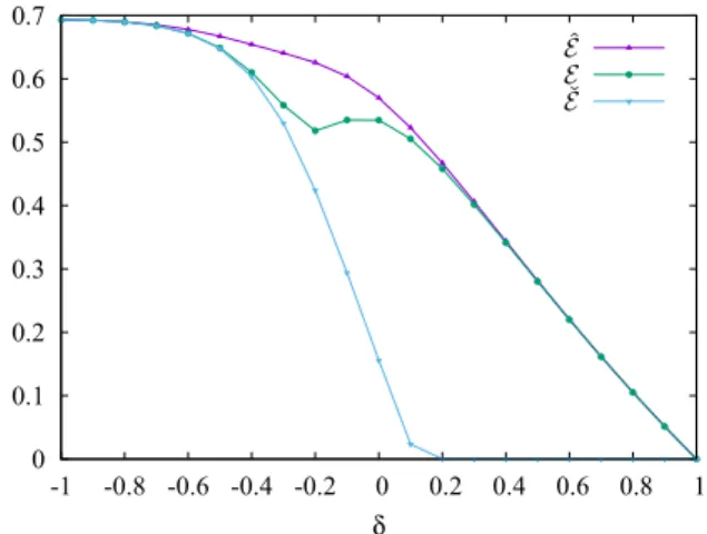
In our first example we consider the ground state of a chain with N =8 and=2. The data are shown in Fig.1 as a function of the dimerization parameterδ. Note that, since N/2=4 is even, the hopping between the two subsystems is given by 1−δ. Thus the entanglement vanishes forδ=1
0 0.1 0.2 0.3 0.4 0.5 0.6 0.7
-1 -0.8 -0.6 -0.4 -0.2 0 0.2 0.4 0.6 0.8 1 δ
FIG. 1. Logarithmic negativity bounds vs exact results in the ground state, as a function of the dimerizationδ, with N=8 and =2.
while it is given by ln 2 at the other extremeδ= −1, where a singlet is formed in the center. As expected from its con- struction, the lower bound ˇE performs well only in the region δ <0, where one has a singlet-type dominant contribution to the entanglement. Remarkably, the upper bound ˆE gives an overall good performance on both sides, with an almost perfect saturation forδ >0.2. However, approaching δ→ −1, the entanglement tends to stay closer to its lower bound.
It is very instructive to have a look also at the thermal case.
Here we consider the two halves of a chain withN =8 sites as subsystems and vary the temperature. This scenario exhibits a very rich physics, as depicted on Fig. 2, where now the symbols show the exact data, whereas the solid lines with matching colors give the respective bounds. In fact, in the regimeδ <0 where the couplings at the boundaries are weak, the Hamiltonian (84) supports edge states. Consequently, the ground state shows topological features which yields an additional ln 2 contribution to the entanglement asδ→ −1.
Since the state is pure, one hasE=Eˆ, as discussed earlier.
0 0.2 0.4 0.6 0.8 1 1.2 1.4
-1 -0.5 0 0.5 1
δ
β=100GS β=5β=2
FIG. 2. Logarithmic negativity bounds vs exact results for thermal states, as a function of the dimerizationδ, and for various values of β. The symbols represent the exact data, while the solid lines with matching colors show the corresponding bounds.
However, already a slight increase of the temperature (see β =100) seems to destroy this order, hence the topological contribution to the entanglement vanishes. Not surprisingly, for these low temperatures, the upper bound gives a very good overall estimation. Nevertheless, for increasing temperatures, the data gradually move towards the lower bound. This im- proved performance can be understood by a simple argument.
The construction of the lower bound erases all the correlations within each subsystem A and B. At higher temperatures, however, such correlations are already washed out and thus the approximation is more valid.
B. Upper bound for infinite homogeneous chain From now on we focus on the homogeneous chainδ =0, and take the thermodynamic limitN → ∞. The Hamiltonian is then diagonalized by a Fourier transform and the correlation matrix takes the simple form
Cm,n= + π
−π
dq 2π
e−i(m−n)
e−βcosq+1. (86) Our main goal is to study the scaling of the upper bound as a function of the inverse temperatureβ and subsystem sizes
|A| =1 and|B| =2 and compare it to the predictions of CFT [22].
1. Ground state
We start with the study of ˆE in the ground state and take 1=2= for simplicity. Invoking Eq. (82), one observes that the upper bound can be written as the difference of two Rényi entropies, with respect to Gaussian statesρA∪Bandρ×. Note that, while the former is just the reduced density operator of an interval of size 2in an infinite hopping chain, the latter one has no particular physical interpretation.
To understand the scaling behavior of the entropies, it is useful to have a look at the corresponding free-fermion entanglement HamiltoniansHandH×, defined by [57]
ρA∪B= e−H
Z , ρ×= e−H×
Z× . (87) Their single-particle spectra, εk and ε×k, respectively, are related via
ζk=tanhεk
2, ζk×=tanhεk×
2 (88)
to the spectra ζk of Gand ζk× of G×. Owing to the simple thermal form (87) of the density operators, the calculation of Renyi entropies reduces to evaluating entropy formulas for a Fermi gas. In fact, the leading contributions to the entropies are delivered by the low-lying eigenvalues of the spectra. For the entanglement HamiltonianH, these were studied before and, for ln1, are given approximately by [58,59]
εk= π2(k−1/2−)
ln(4)−ψ(1/2), (89)
with the digamma functionψ(1/2)≈ −1.963. Thus the entan- glement Hamiltonian has a level spacing inversely proportional to ln, or in other words, a logarithmic density of states. In turn,
-20 -15 -10 -5 0 5 10 15 20
-15 -10 -5 0 5 10 15
ε×k
k-1/2-
=100=50
=200
FIG. 3. Single-particle spectraε×k for various. this yields the celebrated result for the Renyi entropies
Sα(ρA∪B)=1
6(1+α−1) ln+const. (90) We shall now have a look at the spectraε×k and their behavior as a function of , shown in Fig.3. Apart from the double degeneracy of the eigenvalues, the spectra show very similar features to those ofεk. In particular, one can observe the slow logarithmic variation of the spacing and the approximate linear behavior around zero. We thus propose the ansatz
ε×2k−1=ε2k× =aπ2(k−1/2−/2)
ln(2)+b , (91)
with fitting parameters a and b. Fitting the lowest-lying eigenvalue as a function of , we obtain a=1.325≈4/3 andb=1.655 where, for better fit results, we also included a subleading term proportional to 1/. Note that the higher part of the spectrum shows a slight upward bend, which is again very similar to the behavior of theεkspectra [59].
From the ansatz in Eq. (91) it is very easy to infer the leading scaling behavior of the Renyi entropies. Indeed, the main difference from (89) is the increased level spacing, leading to a decrease of the density of states by a factor of a−1≈3/4. Taking into account also the double degeneracy of the spectrum, one arrives at
Sα(ρ×)=1
4(1+α−1) ln+const. (92) That is, ignoring the subleading constant, which is also modi- fied due to the parameterb, the entropiesSα(ρ×) andSα(ρA∪B) differ by a factor of 3/2. This is indeed the result we find numerically by fitting the data for variousα. Finally, inserting the appropriate Renyi entropies into (82), one immediately finds
Eˆ=1
4ln+const. (93)
Thus the upper bound shows exactly the same scaling as the logarithmic negativity predicted by CFT calculations with central chargec=1 [22].
It is instructive to have a look also at the case of unequal adjacent segments of size1and2, where the CFT prediction