A Review on Joint Carotid Intima‑Media Thickness and Plaque Area Measurement in Ultrasound for Cardiovascular/Stroke Risk Monitoring: Artificial Intelligence Framework

(1)

https://doi.org/10.1007/s10278-021-00461-2 REVIEW

A Review on Joint Carotid Intima‑Media Thickness and Plaque Area Measurement in Ultrasound for Cardiovascular/Stroke Risk Monitoring: Artificial Intelligence Framework

Mainak Biswas¹ · Luca Saba² · Tomaž Omerzu³ · Amer M. Johri⁴ · Narendra N. Khanna⁵ · Klaudija Viskovic⁶ · Sophie Mavrogeni⁷ · John R. Laird⁸ · Gyan Pareek⁹ · Martin Miner¹⁰ · Antonella Balestrieri² · Petros P Sfikakis¹¹ · Athanasios Protogerou¹² · Durga Prasanna Misra¹³ · Vikas Agarwal¹³ · George D Kitas^14,15 · Raghu Kolluri¹⁶ · Aditya Sharma¹⁷ · Vijay Viswanathan¹⁸ · Zoltan Ruzsa¹⁹ · Andrew Nicolaides²⁰ · Jasjit S. Suri²¹

Received: 1 July 2020 / Revised: 19 March 2021 / Accepted: 4 May 2021

Abstract

Cardiovascular diseases (CVDs) are the top ten leading causes of death worldwide. Atherosclerosis disease in the arteries is the main cause of the CVD, leading to myocardial infarction and stroke. The two primary image-based phenotypes used for monitoring the atherosclerosis burden is carotid intima-media thickness (cIMT) and plaque area (PA). Earlier segmentation and measurement methods were based on ad hoc conventional and semi-automated digital imaging solutions, which are unre- liable, tedious, slow, and not robust. This study reviews the modern and automated methods such as artificial intelligence (AI)- based. Machine learning (ML) and deep learning (DL) can provide automated techniques in the detection and measurement of cIMT and PA from carotid vascular images. Both ML and DL techniques are examples of supervised learning, i.e., learn from “ground truth” images and transformation of test images that are not part of the training. This review summarizes (1) the evolution and impact of the fast-changing AI technology on cIMT/PA measurement, (2) the mathematical representations of ML/DL methods, and (3) segmentation approaches for cIMT/PA regions in carotid scans based for (a) region-of-interest detection and (b) lumen-intima and media-adventitia interface detection using ML/DL frameworks. AI-based methods for cIMT/PA segmentation have emerged for CVD/stroke risk monitoring and may expand to the recommended parameters for atherosclerosis assessment by carotid ultrasound.

Keywords Atherosclerosis · Carotid ultrasound · Plaque · Artificial intelligence · Machine learning · Deep learning · Carotid intima-media thickness · Carotid plaque area

Introduction

Cardiovascular disease (CVD)-related deaths in the United States of America (USA) were 17.6 million in 2016, and that is 14.5% higher than reported in 2006 [1]. The major causes of such an increase in fatalities can be attributed to an increase in tobacco use, physical inactivity, obesity, high blood pressure, diabetes, arthritis, coronary artery disease, and other disorders. This has deep economic implications on the US economy. It is estimated that the total direct and indirect costs were US $351.2B in 2014–2015, adjusting to inflation [1, 2].

The main cause of CVD is the blood vessel inflamma- tory disease, called atherosclerosis [3, 4]. Atherosclerosis is initiated by endothelium dysfunction [4, 5], where the thin wall of the interior surface of blood vessels gets dam- aged leading to the formation of more complex lesions and fatty streak within arterial walls [1, 6–8]. Several studies have been conducted demonstrating how atherosclerosis progresses in the carotid arteries. One study on 68 asymptomatic patients with greater than 50% stenosis showed that the wall area increased by 2.2% per year over 18 months [9]. Another study that ran over 22±15 months, consisting of 250 patients with asymptomatic plaques having 40–99%

stenosis, showed a high percentage area of lipid-like mat- ter. This risk factor caused subsequent cerebral infarction (hazard ratio = 4.4) [10]. Such a situation generally signi- fies a time bomb where the artery can no longer sustain the

* Jasjit S. Suri

Jasjit.Suri@AtheroPoint.com

Extended author information available on the last page of the article

/ Published online: 2 June 2021

(2)

plaque burden leading to the rupture of the fibrous cap. This leads to the intrusion of plaque into the bloodstream causing thrombosis and finally resulting in a stroke [11–13] (shown in Fig. 1). Atherosclerosis has been also linked to neuronal diseases such as dementia [14], leukoaraiosis [15, 16], and Alzheimer’s [17], renal diseases [18, 19], arthritis [20], and coronary artery diseases [21].

The atherosclerotic disease can be quantified by tracking the carotid intima-media thickness (cIMT) and plaque area (PA) over time, so-called atherosclerotic disease monitoring or vascular screening [22]. The cIMT is the measured distance between lumen-intima (LI) and media-adventitia (MA) borders [23, 24] while the area covered between the LI and MA boundary walls typically refers to PA [25–32]. The role of cIMT/PA measurement has gone beyond is normal tracking of the atherosclerosis burden, but rather computing CVD composite risk estimation, unlike the traditional risk calculators such as Framingham [33], ASCVD [34], Reynold risk score (RRS) [35], United Kingdom Prospective Diabetes Study (UKPDS56) [36], UKPDS60 [37], QRISK2 [38], and Joint British Societies (JBS3) [39]. None of these conventional calculators used plaque burden as a risk factor. This changed recently when AtheroEdge Composite Risk Score (AECRS 1.0) [20] was developed that used an automated morphological-based CVD risk prediction tool that integrates both conventional and imaging-based phenotypes such as cIMT and PA. The image-based biomarkers are based on the scanning of carotid segments such as a common carotid artery, bulb, or internal carotid artery acquired using 2D B-mode ultrasound [5, 40, 41]. AECRS 2.0 is another class of image-based 10-year risk calculator that combines conventional risk factors, blood biomarkers,

and image-based phenotypes. It is these image-based phenotypes that are an integral part of the risk calculators, and therefore, better understanding is needed on how cIMT/PA can be computed automatically in artificial intelligence (AI) framework. To get a better idea, one must therefore see how the cIMT/PA evolved over time.

There are different school-of-thoughts (SOT) dealing with automated identification of the cIMT/PA region (so-called segmentation) for static (or frozen) and motion images;

however, the scope of this work is only limited to static scans. These SOTs range from simple image morphology- based threshold techniques to deep learning (DL)-based AI systems developed over 50 years. Therefore, a generation- wise categorization is necessary. Thus, SOTs can be further divided into three generations based on how the ROI region is determined [42] and then how LI/MA is searched in this ROI region. The first-generation technologies were low-level segmentation techniques which used conventional image processing methods based on the primary threshold to get the edges of LI/MA and then use a caliper-based solution to measure the mean distance. The second-generation (or second kind of methods) used contour-based methods, which consisted of parametric curves or geometric curves. Some of these methods are semi-automated [43–46]. Further in the same class were a fusion of signal-processing-based methods (such as scale-space) and deformable models. These were categorized under the class of AtheroEdge™ models. They are completely and fully automated. Some methods were regional-based combined with deformable models under the fusion category in generation 2. These were also fully automated [47, 48]. The latest third-generation models use AI technology like machine learning (ML) [49] and DL [50]

Fig. 1 (i) Left panel: atherosclerosis progression consisting of (a) endothelium dysfunction and lesion initiation, (b) formation of a fatty streak, (c) formation of fibrous plaque underlying fibrous cap, and (d)

rupture and thrombosis. (ii) Right panel: ultrasound scanning of the carotid artery (both images courtesy of AtheroPoint™, Roseville, CA, USA)

(3)

for both ROI estimation and LI/MA interface detection. All the three generations used some kind of distance measurement method such as shortest distance, centerline distance, Hausdorff distance [51], and more often adapted and called as “Suri’s polyline distance method” [52]. This review is focused on how ML and DL can be used for cIMT/PA measurements, which in turn requires LI/MA detection in plaque and non-plaque regions.

The layout of the paper is given as follows: the “Chrono- logical Generations of cIMT Regional Segmentation and cIMT Measurement” section gives an overall overview of conventional and advanced techniques in joint carotid cIMT/PA estimation along with their classification. The

“ML Application for cIMT and PA Measurement” section is dedicated to both ML and DL techniques applied for the segmentation of cIMT/PA regions. The “Deep Learning Application for cIMT and PA extraction” section provides different quantification techniques, and finally, the paper concludes in the “Discussion” section.

Chronological Generations of cIMT Regional Segmentation and cIMT Measurement

As already known, the carotid IMT is the surrogate biomarker for carotid/coronary artery disease [53]. Several first- generation computer vision and image-processing techniques have been developed for the low-level segmentation of the cIMT region (the region between LI and MA borders) and LI/MA interface detection, such as dynamic programming (DP) [54], Hough transform (HT) [55], Nakagami mixture modeling [56], active contour [57], edge detection [58], and gradient-based techniques [59].

These come under the class of computer-aided diagnosis [40, 60, 61]. The comparison of these methods has been presented previously [62–66]. Dynamic programming uses optimization techniques to minimize the cost function which is the summation of weighted terms of local estimations such as echo intensity, intensity gradient, and boundary continu- ity. All sets of spatial pixel points forming a polyline are considered. The polyline having the lowest cost is considered the cIMT vertices and such polylines constitute the boundary [54]. The HT of a line is a point in the (s, θ) plane where all the points on this line map into this single point.

This fact is utilized to find different line segments through edge points which can be used to detect curves in an image.

HT has been used for lumen segmentation in various works by Golemati et al. [67], Stoitis et al. [68], and Petroudi et al.

[69], and Destrempes et al. [56] used Nakagami distribution and motion estimation to segment the cIMT region. This generation also involved the usage of signal processing techniques such as scale-space [70] to detect LI and MA boundaries [46]. Several version of cIMT segmentation methods

with scale-space based augmented by second-generation methods (so-called [24, 71–73]).

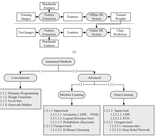
In the second generation, the concept of active contour evolved that involves fitting a contour to local image information. Snakes or active contour are an example of active parametric contours [14] that were used for LI/MA estimation, followed by cIMT measurement [74]. In the same class, curve fitting models were a classic example of the cIMT estimation method [75]. Level sets topologically independent propagating zero level curves to settle at the interfaces of LI and MA were used to compute the LI/MA interfaces so- called as cIMT borders [76]. There has been a method which fuses first generation and second generation, such as fusion of scale-space [70] with deformable models [46]. Several version of cIMT segmentation methods with scale-space based augmented by second-generation methods (so-called [24, 71–73]). Edge detection techniques use a variation of grey levels and included image gradient to delineate cIMT borders [77]. Molinari et al. used a fusion of these approaches to segment the cIMT borders [78]. Elisa et al. [27] used an automated software AtheroEdge™ system [19, 66, 79] based on scale-space for computing cIMT and plaque area (PA) after computing LI-and MA boundary interfaces. The third- generation advanced techniques consist of intelligence-based techniques such as ML [49] and DL [50] techniques, primar- ily banking on neural network models. ML was based on hand-crafted features, while DL was more along the lines of automated feature extraction. Regarding the risk prediction of CVD, both ML and DL have been objective and methodologies that can be replicated with high diagnostic accuracy [80, 81]. A representation of technologies generation wise is shown in Fig. 2. A detailed discussion of general working of ML and DL follows next.

ML and DL differ in the methodology of feature derivation from instances. In the case of ML (details in Appendix 1), feature extraction is independent of the actual model of classification and is handcrafted (shown in Fig. 3 (i)), whereas, in DL, the feature extraction and model of characterization are indifferent from each other. ML models of classification mostly appear as a single statistical learning and inference technique to make accurate predictions using the extracted features [82, 83]. The DL models, on the other hand, apply multiple layers of statistical learning and inference techniques to extract features and make predictions. Hence, the DL techniques are costlier in terms of computation time and space, but are more robust and in some cases provide higher accuracy, when applied to a very large dataset [84]. ML techniques are more economical in both time and cost when compared with DL. Often these two techniques are clubbed together for better performance. An interesting characteristic is how ultrasound image noise (speckle noise, scattering noise) was handled by each of these generations. While the first two generations used various denoising techniques such as Gaussian filter,

(4)

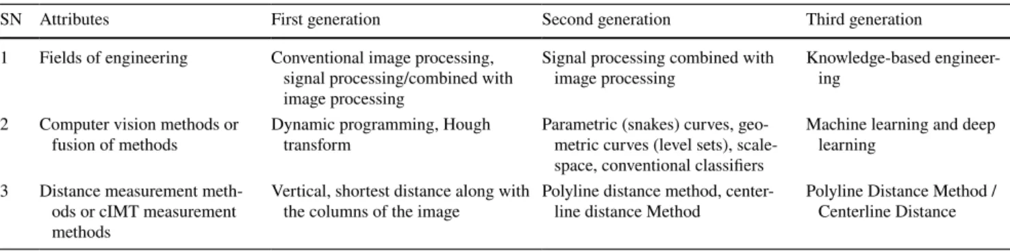
anisotropic diffusion, and smoothing, there was no evolution of such in third-generation [64, 65, 75, 85]. A brief outline of technologies generation wise is given in Table 1. Although technologies were divided generation wise, they were not water-tight compartments. Many models were a fusion of different technologies belonging to different generations to increase performance. In this regard, Molinari et al. [23] used a combination of first and second techniques to minimize the cIMT error.

The PA biomarker received significant research focus after it was conclusively proven to be as important as cIMT in the works of Spence et al. [86, 87], Mathiesen et al. [88], and Saba et al. [79]. Mathematically, PA can be computed along with cIMT if LI/MA borders are known. It is computed by counting all pixels between LI and MA borders and then calibrating it to mm². PA has been well adapted in AECRS 1.0 [89] and AECRS2.0 [18] systems.

ML Application for cIMT and PA Measurement

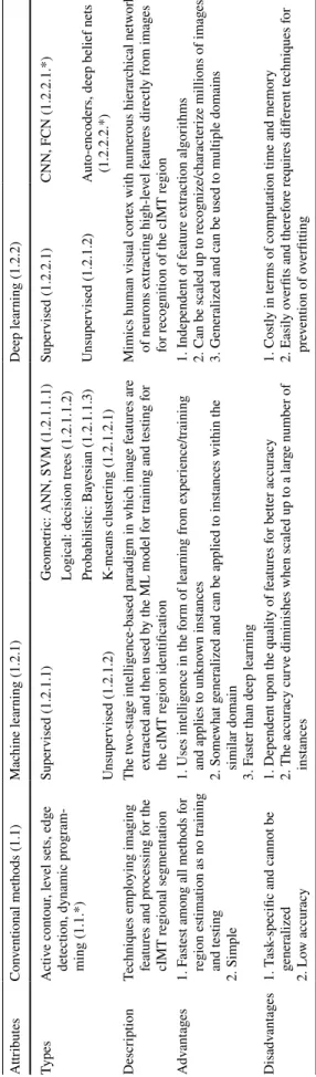
In the Appendix 1, a brief outline of ML techniques was given. The different AI methodologies are shown in Fig. 3 (ii) and their description is given in Table 2. This is categorized into conventional, machine learning, and deep

learning strategies. In this section, we will study in detail about different ML techniques that are applied for cIMT/

PA segmentation and measurements from CCA images. As stated earlier, features are needed to be extracted before the ML model is applied. Some part of the features is used for training the model, i.e., training data ( X_tr) , while the rest of it is used to test the model, i.e., test data (X_ts ). The training process uses a feedback mechanism based on known and actual outputs, wherein the model parameters are changed based on the error. This training process repeats until the model parameters converge or do not change their values anymore, it is conceded that training is complete. There- fore, the model with trained parameters is tested on X_ts with outputs unknown to the model. Once model outputs are out, they are compared with actual outputs to check the performance of the model. Several applications of ML has been developed which uses the concept of offline and online system, such as arrhythmia [90] and diabetes [91].

Since they all use ground truth during cross-validation, we call them supervised learning, and is applied extensively in cIMT and PA computation from CCA images. There are two different SOTs (Rosa et al. [92, 93] and Molinari et al.

[23]) regarding segmenting the cIMT region from ultrasound CCA images. Both SOTs extract the ROI before the application of ML paradigm for cIMT segmentation. They are given as follows:

Fig. 2 Three generations of cIMT/PA measurement evolution (color image) (courtesy of AtheroPoint™, Roseville, CA, USA)

Table 1 The three generations of cIMT regional segmentation

SN Attributes First generation Second generation Third generation

1 Fields of engineering Conventional image processing, signal processing/combined with image processing

Signal processing combined with

image processing Knowledge-based engineering

2 Computer vision methods or

fusion of methods Dynamic programming, Hough

transform Parametric (snakes) curves, geo-

metric curves (level sets), scale- space, conventional classifiers

Machine learning and deep learning

3 Distance measurement methods or cIMT measurement methods

Vertical, shortest distance along with

the columns of the image Polyline distance method, center-

line distance Method Polyline Distance Method / Centerline Distance

(5)

ANN Model for cIMT Region Detection

Rosa et al. [92] used three stages to acquire cIMT values from 60 B-mode ultrasound CCA images. In stage I, the CCA images were preprocessed to extract ROI, and stage-II is the AI-based classification stage where the IMT regional pixels were segregated from non-IMT regional pixels resulting in a binary image. Stage III consisted of delineation of LI and MA boundary from the binary image. The preprocessing stage consisted of the application of watershed transform [94–96] of the CCA to detect the lumen, wherein the lower limit of the lumen is assigned as the posterior wall. The final ROI in the region, where the uppermost point of the far wall was considered as 0.6 mm above the binary lumen, and the bottom boundary is fixed to 1.5 mm below the lowest point detected in the binary mask. Once the ROI is detected, its dimension is noted and extracted from the original image as shown in Fig. 4 (i). The extracted ROIs are input to the next stage for IMT border delineation. The next stage applies the ensemble of four artificial neural networks (ANNs) [97] to classify cIMT from non- cIMT region pixels. The ANN is in the form of a multi-layer perceptron consisting of three layers such as input, hidden, and output as shown in Fig. 4 (ii). In the ANN model, the computation is done by the nodes, whereas the “learning experience”

is embedded in the weights between input-hidden and hidden- output layers. These weights generally are randomly initialized and converge to a stable value based on the feedback on the error propagation as the learning progresses. The computation is generally, multiplication of weights with the input values, thereafter, a sigmoid function (𝜎= ¹

1+e^−x) is applied. Also, a bias term 𝛽 is added to each computed term. The output function is given by:

where i and j signify the weights between input-hidden, and hidden-output layers, respectively. The weight values ( w_ij ) are optimized for each error propagation using the gradient ( _Δw^Δ𝜀 ), given as:

where 𝛾 is the learning parameter. The input pattern to each ANN is the pixel intensities that are generated by a kernel process. For each image, three kernels of size 3 × 3, 7 × 7, and 11 × 11 were applied pixel-by-pixel through shifting, to collect contextual information of neighborhood pixel intensities. The process is also known as convolution and its operation using the 3×3 kernel is shown in Fig. 4 (iii).

The ground truth was the pixel class information collected through manual segmentation of CCA images and annota- tion of each pixel being cIMT boundary or not. Therefore, the inputs were passed through three ANNs, respectively,

̂f(x) =𝜎( (1)

𝛽^jy+W^jy(𝜎(𝛽^ij+W^ij)))

(2) w_ij=w_ij−𝛾Δ𝜀

Δw

Table 2 Comparison between different cIMT regional segmentation methods for given attributes AttributesConventional methods (1.1)Machine learning (1.2.1)Deep learning (1.2.2) TypesActive contour, level sets, edge detection, dynamic programming (1.1.*)

Supervised (1.2.1.1)Geometric: ANN, SVM (1.2.1.1.1)Supervised (1.2.2.1)CNN, FCN (1.2.2.1.*) Logical: decision trees (1.2.1.1.2) Probabilistic: Bayesian (1.2.1.1.3)Unsupervised (1.2.1.2)Auto-encoders, deep belief nets (1.2.2.2.*)Unsupervised (1.2.1.2)K-means clustering (1.2.1.2.1) DescriptionTechniques employing imaging features and processing for the cIMT regional segmentation

The two-stage intelligence-based paradigm in which image features are extracted and then used by the ML model for training and testing for the cIMT region identification

Mimics human visual cortex with numerous hierarchical network of neurons extracting high-level features directly from images for recognition of the cIMT region Advantages1. Fastest among all methods for region estimation as no training and testing 2. Simple

1. Uses intelligence in the form of learning from experience/training and applies to unknown instances 2. Somewhat generalized and can be applied to instances within the

similar domain 3. Faster than deep learning

1. Independent of feature extraction algorithms 2. Can be scaled up to recognize/characterize millions of images 3. Generalized and can be used to multiple domains Disadvantages1. Task-specific and cannot be generalized 2. Low accuracy

1. Dependent upon the quality of features for better accuracy 2. The accuracy curve diminishes when scaled up to a large number of instances

1. Costly in terms of computation time and memory 2. Easily overfits and therefore requires different techniques for prevention of overfitting

(6)

for training and testing. The output is in the form of another reconstructed binary image from each of the three ANNs.

Thereafter, these three output binary images are merged and another kernel of size 3 × 3 is again applied to the merged image and this data is fed into the fourth ANN to get the final binary mask. A representative model of the entire process is shown in Fig. 4 (iv). In the final stage, LI and MA boundaries are identified (shown in Fig. 4 (v)) and cIMT is computed. The mean absolute distance, polyline distance, and centerline distance were 0.03763±0.02518 mm, 0.03670±0.02429 mm, and 0.03683±0.02450 mm, respectively.

Extreme Learning Machines‑Radial Basis Neural Network Model for cIMT Region Detection

Rosa et al. [93] used radial basis neural network (RBNN) [98] for the estimation of the cIMT region from 25 ultrasound CCA images. RBNNs are single-layer feed-forward neural networks consisting of input, hidden, and output layers. One of the key differences between RBNN and ANN is that the number of hidden layers in RBNN is restricted to one. The working principle of RBNN lies in interpolating r training points x^r to their corresponding target variable

y^r . Therefore, the model output function for an input x^ts is given by:

where 𝜑_r is the Gaussian radial basis function implemented by the hidden layer, w_r is the weight between the hidden and output layer. The 𝜑_r is the radial basis function which is given by:

where 𝜌 represents the width of the hidden neuron. Equa- tion (3) can be reduced into a matrix notation and is given as:

where T is the target vector. The weights can be found by standard matrix inversion

the initialization of hidden nodes’ Gaussian parameters (number of hidden nodes, centers, and deviation of each radial unit) are done using optimally pruned-extreme (3)

̂f(x) =∑N

r=1w_r𝜑_r(⇑x^ts−x^r⇑)

(4) 𝜑_r�

‖x^ts−x^r‖�

=exp

�‖x^ts−x^r‖² 2𝜌²

�

(5) W𝝋=T

(6) W =𝝋⁻¹T

Fig. 3 (i) Generalized ML model and (ii) classification tree of different automated models

(7)

learning machine (OP-ELM) [99, 100]. The ground truth information and ROI of the 25 CCA images are extracted using the method mentioned in the “ANN Model for cIMT Region Detection” section. Similar to the previous method [92], the input pattern is generated by the kernel process. A comparative study was performed using varying kernel sizes in the range of 3 to 23. The optimized kernel window size was 19×19 . The ground truth was manually traced by experienced radiologists. Three classes of pixels were considered for each CCA image, pixels of the LI boundary, pixels within the region between LI and MA boundary, and the pixels of

the MA wall. Finally, each class of pixels were extracted and superimposed on the original image as shown in Fig. 4 (vi).

The cIMT error for this experiment was 0.065±0.046 mm.

Fuzzy K‑means Classifier for cIMT Region Extraction Molinari et al. [23] introduced the concept of unsupervised learning of fuzzy K-means clustering [101] (FKMC) to seg- regate a CCA image into three parts, i.e., plaque region, LI, and MA boundaries. This method is also called CULEX_ia. The FKMC is unsupervised in the sense that there is no

Fig. 4 (i) ROI extraction (reproduced with permission), (ii) ANN, (iii) convolution operation, (iv) stage II ANN ensemble network, (v) outputs of [92] (reproduced with permission), (vi) segmentation using RBNN [93] (reproduced with permission)

(8)

ground truth for the pixels. The FKMC is similar to the K-means algorithm [102], where initially K random points denoting K cluster centers are initialized, and then all data points in the dataset are assigned to each of the K clusters based on the nearest mean. For each cluster centroid, c_j represents the mean of all points in the cluster. The membership function b_ij of each point a_i determining degree of its membership for each cluster c_j , is given by:

where m is a hyper-parameter controlling fuzziness.

In this work, the ROI is extracted from each CCA image by tracing the MA wall. The MA wall is traced by locat- ing the brightest local maximum starting from the bottom of the image for each column. The upper limit of ROI is computed 1.25 mm and 0.625 mm above and below the MA wall, respectively as shown in Fig. 5 (i). Thereafter, in the next stage, three clusters of pixels are considered for each column in the ROI column-wise, i.e., lumen, LI, and MA wall. The pixels in each column are automatically assigned to each cluster using the FKMC algorithm. The sequence of LI and MA centroids for each column marks the delineation of respective walls in the ROI as shown in Fig. 5 (ii). This procedure was repeated for 200 ultrasound CCA images.

The cIMT error for the method was 0.054±0.035 mm. The ML models discussed covered cIMT measurement in brief;

however, they did not consider plaque area until the DL work by Elisa et al. [103] in 2018 and joint cIMT and PA measurement by Biswas et al. [104] in 2020. A brief outline of DL in cIMT and PA measurement is given in the next section.

Deep Learning Application for cIMT and PA Extraction

There are several DL techniques used for image classification and segmentation [82, 105] such as CNN [50], deep belief networks (DBN) [106], autoencoders [107], and residual neural networks [108]. Fully convolutional network (FCN) [109] is a variation of CNN which excludes the connected network and is used specifically for segmentation. Three different SOTs are working on cIMT measurement using ultrasound CCA images. DL. Rosa et al. [110] used autoencoders for feature extraction before employing ANNs for LI and MA boundary delineation. Suri and his team used FCN both on whole [111] and patch [104] CCA ultrasound images for cIMT and PA [103] measurement while Del Mar et al. [112] used FCN for whole CCA images for cIMT estimation. The next few subsections deal with some of these works in detail for cIMT and PA measurement computed using CCA images.

b_ij= 1 (7)

�∑^K

k=1

‖a_i−c_j‖

‖a_i−c_k‖

�_m−1² 0≤b_ij≤1

ANN Autoencoder‑Based cIMT Region Segmentation Rosa et al. [110] used ANN for characterizing LI and MA pixels belonging to 55 ultrasound CCA images. The authors used trained autoencoders [107] to extract features in the LI and MA interface. Autoencoders are neural networks designed to reproduce the input. They are generally used for unsupervised learning to understand complex relationships within input images. Given an input ∈ [0,1]^dx , the autoencoder maps it to a compressed representation using single or multiple hidden layers,Y∈ [0,1]^dy using the mapping function similar to Eq. 3. Finally, the compressed representation is upsampled to its original dimension. It is done so to understand the essential structures and relationships with the input vector, and the training required to regenerate it. The compressed representation of neighborhood pixels denotes the features. An illustration of the autoencoder is shown in Fig. 6 (i). The ROI extraction approach is similar to [92].

The authors trained two autoencoders using five ground truth images. The neighborhood pixels of the LI and MA interface were used to train the two autoencoders. The LI and MA features were used to train two ANNs for pixel characterization. Finally, the offline CCA images were segmented, to extract the LI and MA boundary. Postprocessing was applied to discard the unnecessary LI and MA pixels. The system’s cIMT error was 0.0499±0.0498 mm. The process model is shown in Fig. 6 (ii) while the results are shown in Fig. 6 (iii).

Fully Convolutional Network for cIMT Region Estimation

In the work by Biswas et al. [111], the LI and MA borders were extracted in three stages from 396 ultrasound CCA images. The ground truth was binary images obtained from tracings of LI and MA borders by two experienced radiologists using general- purpose tracing software AtheroEdge™ [66, 113, 114]. In the first multiresolution stage, the images were cropped 10% from each side to ensure that the low-contrast and the nonrelevant por- tion of the images do not affect learning in the second stage.

This typically arises due to poor probe-to-neck contact or lack of gel during the image acquisition. In the second stage, FCN was applied to segment the cIMT region from the rest of the image. The FCN-based system consisted of two subsystems: (i) encoder and decoder (shown in Fig. 7 (i)). The encoder consisted of 13 layers of convolution (two layers of 64 (window size = 3 × 3) kernels + two layers of 128 (window size = 3 × 3) kernels + three layers of 256 (window size = 3 × 3) kernels + three layers of 512 (window size = 3 × 3) kernels + three layers of 512 (window size = 3 × 3) kernels), and five max-pooling layers to draw a downsampled representation or feature map of the image.

The convolution operation (similar to as discussed in Sect. 3.1 by Rosa et al. [92]) applies kernel filters over the image pixel- by-pixel to extract contextual information and position invariant

(9)

features of the cIMT wall region. Before every max-pooling operation, a 1 × 1 convolution operation is employed to reduce the feature maps to a single map. The decoder constitutes three upsampling layers to upsample the downsampled feature map, two intermediate skipping operations to merge intermediate feature maps and one softmax layer to make pixel-to-pixel comparison with the ground truth. Mathematically, the convolution operation is given as:

where g is the output representation at the location (a,b), I is the input image, k is the kernel of size m×m , (a,b) represents the location of the pixel, and (s,t) are dummy variables.

The max-pooling operation is used for the downsampling of the feature map by retaining the most important information from each block of the image. The FCN model applied is shown in Fig. 7 (i). The encoder applies 13 layers of convolution (shown in red boxes), five max-pooling layers (shown in blue boxes) to obtain a feature map of (1/32^nd) size of the original image as shown in Fig. 7 (i).The decoder using a series of three up-sampling layers (shown in gray boxes) and intermediate skipping operations (shown in green boxes) to perform dense softmax classification (shown in the orange box) with ground truth for each feature map pixel. The upsampling operation is the inverse of convolution applied to the feature map at the end of the encoder. Three up-sampling layers were applied to expand the image to its original size.

The skipping operations merged features maps from con- tracting layers of the encoder to the intermediate layers of

(8) g(a,b) =I(a,b)⊗k(a,b) =∑^m₂

s=−^m

2

∑^m₂

t=−^m

2

I(a+s,b+t) ×k(a,b)

the decoder to recover spatial information lost during the downsampling in the encoder. The cross-entropy loss function for the pixel-to-pixel characterization is given by:

where 𝛼₁ is the prediction, 𝛼₂ is the gold standard or GT, L is the total number of classes, and N is the total number of images. The softmax layer is used for final characterization where a pixel is assigned a class with the highest probability as given by:

where z_i represents the output score of the instance for the ith class. The segmented images were computed by fixing the DL iterations to 20,000. Finally, in the third stage, refine- ment of MA boundary was done using calibration employing a matrix inverse operation [115]. The LI and MA borders along with their ground truth counterpart are shown in Fig. 7 (ii). The cIMT error obtained for this application using DL on the two ground truth values were 0.126±0.134 and 0.124±0.10 mm, respectively.

FCN for PA Measurement

Elisa et al. [103] used a similar strategy [111] discussed in the “ANN Autoencoder-Based cIMT Region Segmentation”

section, to obtain the PA values for the same cohort using the same ground truth and drew important conclusions. The (9) 𝜃_class(𝛼₁,𝛼₂) = 1

�N�

∑

n∈N

∑

l∈L𝛼_2n(l)log𝛼_1n(l)

P� (10) z_i�

= e^zⁱ

∑N j=1e^z^j

Fig. 5 (i) Far wall detection and (ii) segmentation of LI (white) and MA (black) boundary (reproduced with permission) [23]

(10)

PA error values for the two ground truth values were 20.52 mm² and 19.44 mm², respectively. The coefficient of correla- tion between PA and cIMT using the outputs of DL for the two ground truths were 0.92(p<0.001) and 0.94(p<0.001) , respectively. The output image is shown in Fig. 7 (iii).

Two‑Stage Patching‑Based AI Model for cIMT and PA Measurement

Recently, Biswas et al. [104] used a two-stage DL-based network for cIMT and PA measurement. In the first stage, a CNN was applied for extraction of ROI while in the second stage, an FCN similar to [111] was used for delineation of LI and MA borders and cIMT measurement. CNN is different from FCN in the way that CNN applies a neural network in the form of a fully connected layer for classification, whereas a trained

FCN only applies convolution and subsequently upsampling to regenerate a feature map representing semantic segmentation of the actual image. A representative diagram of the 2-layer CNN model is shown in Fig. 8 (i). The softmax classification function (Eq. 12) is used for final characterization for the image. In this work, authors have used 22-deep layers [116] for the extraction of high-level features from the images. Initially, 250 CCA images of the diabetic cohort were collected. A preprocessing was performed using the Athe- roEdge™ (AtheroPoint™, Roseville, CA, USA) system to crop the image to remove background information and ensure the lumen region is central to the cropped CCA image. The resultant cropped CCA image is split horizontally into two halves. The bottom half of the image consisting of the far- wall is taken out and further spit horizontally. The upper split in the bottom half consists of wall information whereas the

Fig. 6 (i) An autoencoder, (ii) process model, (iii) image outputs (reproduced with permission) [110]

(11)

GT LI-Far (Yellow dotted) DL LI-Far (Red line)

GT MA-Far (Yellow dotted) DL MA-Far (Green line)

(a) Original image (b) Plaque Area

(i) The combination of encoder-decoder blocks in the central DL system (a class of AtheroEdge™ system, courtesy of AtheroPoint, CA, USA).

(ii) The DL-based system showing GT (yellow) and DL (green and red) outputs (image courtesy

AtheroPoint^TM, CA, USA).

(iii) (a) Raw input image, (b) LI (RED), MA borders and corresponding ground truth (yellow) borders.

Fig. 7 (i) FCN model, (ii) IMT output using the FCN [111], and (iii) TPA output using the FCN [103]

(12)

lower split consisted of the tissue region. Both the upper and lower splits are divided column-wise into sixteen equal-sized patches. The patches form the input to the two-stage DL-based system. In the first stage, an independent 22-layered CNN network [116] is applied to characterize the input images into the wall and nonwall patches. The CNN accuracy performance for characterization was approximately 99.5%. Once the patches are characterized, the wall patches are combined patient-wise to generate the ROI segment. The preprocessing and DL stage I inputs and outputs are shown in Fig. 8 (ii). These ROI segments along with their binary ground truths are used to train the second stage DL. The second stage DL architecture is similar to the previous architecture [111]. Once trained, the second stage DL system partitions the ROI segment into plaque and nonplaque regions.

Thereafter, LI and MA boundaries are delineated from the plaque region, and cIMT and TPA are computed as shown in Fig. 8 (iii). The cIMT error, PA, and PA error was found to be 0.0935±0.0637 mm, 21.5794±7.9975 mm², and 2.7939±2.3702 mm², respectively. A similar strategy [112]

was applied to the whole CCA images using DenseNet [108]

for the whole 331 images with cIMT mean error 0.02 mm.

Although the DL techniques are accurate, robust, and more scalable than ML techniques, the storage and computation costs are much higher. The several layers of neurons mean a huge number of parallel computations that need to take place which may not be possible in desktop CPU architectures but need graphic processor units (GPUs). Also, the storing of intermediate values requires a huge amount of memory space.

Therefore, ML is more suited to small systems where faster results are needed and accuracy is not a high priority. DL on the other hand suited for industrial medical imaging purposes where there are large patient volumes and higher accuracy is a requirement.

Discussion

In this study, we have looked at several state-of-art AI techniques implemented in recent years for plaque burden quantification in the form of cIMT and PA using carotid ultrasound images. Although AI is a newer concept, it has a significant impact on the medical imaging industry due to its robustness and accuracy. The ML techniques introduced the notion of learning from training images which have been taken over by DL techniques recently.

Even though forthcoming deep learning systems are supe- rior to older stage systems, there is a price to pay on the hardware cost or computational time. We have yet to see more through comparison in terms of speed, accuracy, large cohort, and variability in the resolution of the carotid scans, applied to both CCA and bulb segments. In some works such as application of DL in liver implemented

previously, it has been seen that the presence of noise or redundant information can affect the performance of deep learning significantly [117]. Hence, cropping was done to achieve significant performance levels. The training data size also significantly affects the training performance irre- spective of the cross-validation protocol. A large training pool is always better for training DL models as it captures wider complexities and intricacies of the data pool. This helps in better performance when applied to unknown data. Further, this review sheds light on three generations of cIMT/PA evolution, followed in-depth analysis on several key ML and DL paradigms that computed cIMT and PA values directly from carotid ultrasound images without any human intervention. Note that since the scope of this study was meant for only static (or frozen) ultrasound scans, there was no attempt to study cIMT/PA in motion imagery. However, studies have been done using conventional (non-AI) methods for cIMT estimation in selected frames of the cardiac cycle for understanding the plaque movement [118–120]. A visual comparison of the Athe- roEdge™, a patented software [121, 122], scale-space method [46], and AI-based model (Biswas et al. [111]) is shown in Fig. 9. The AtheroEdge™ model is based on splines and elastic contour and achieved fairly good results, and clear border tracing is achieved. However, it fails around noisy corners. On the other hand, a distinct and clear delineation is achieved by the AI model when compared with the scale-space model. The proposed AI model results are more aligned along the ground truth than the scale-space model for the same patient. The AI model parameters are trained to align along the LI-far and MA- far wall over several iterations leading to better learning.

The better training means that the parameters have also included plausible noise around the walls and got around them to delineate correct borders. Low-level segmentation models such as scale-space have failed to include the noisy information in their computation and therefore give a lesser accurate delineation.

Benchmarking

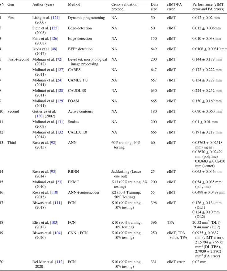
The first- and second-generation techniques have been already briefly described by Molinari et al. [123]. In this section, we have presented Table 3 which shows the benchmarking table using first-, second- and third- generation techniques used in the last two decades. The first-generation techniques are discussed first. In the year 2000, Liang et al. [124] used DP to quantify cIMT from 50 images. Both Stein et al. [125] and Faita et al. [126]

used edge detection techniques to measure cIMT from 50 and 150 CCA images, respectively, with cIMT error of 0.012±0.006 mm and 0.010±0.038 mm , respectively.

(13)

Ikeda et al. [48] used bulb edge point detection technique to quantify cIMT from 649 images with bias between predicted and ground truth being 0.0106±0.00310 mm .

A fusion of first- and second-generation techniques are discussed next. Molinari et al. [72] used a combination of level set and morphological image processing (i) A convolution neural network (courtesy of AtheroPoint™,

CA, USA).

Bottom half Non-Wall Patches

Wall Segment

Non-Wall Segment

First Split Second Split (Horizontal) Third Split (Vertical) Cropped Image using AtheroEdge

Original Image

(a) (b) (c) (d) (e)

Wall Patches

Wall Segment after Reconstruction(f) (ii) Preprocessing and characterization input and output, preprocessing: (a) original CCA image,

(b) cropping using AtheroEdge^TM, (c) first horizontal partition, (d) second horizontal partition, (e) patching, stage-I characterization and reconstruction: (f) extracted ROI segment (image courtesy:

AtheroPoint^TM).

(f) (e)

(c) (d) (a) (b)

Low Risk

Medium Risk

High Risk

(iii) Stage-II DL output, yellow dotted line represents the ground truth LI-and MA borders, red and green line marks the deep learning LI-and MA-walls respectively (image courtesy:

AtheroPoint^TM).

Fig. 8 (i) A CNN model, (ii) patching and reconstruction process, and (ii) outputs of the two-stage DL model [104]

(14)

to estimate cIMT from 200 images. The cIMT error was found to be 0.144±0.179 mm. A similar fusion based patented techniques were developed by Molinari et al. in form of CARES [127], CAMES [24], CAU- DLES [128], and FOAM [129], for cIMT estimation.

The cIMT error for each of them were found to be 0.172±0.222 mm , 0.154±0.227 mm , 0.224±0.252 mm , and 0.150±0.169 mm from 647, 657, 630, and 665 images, respectively. Some of the second-generation techniques that were developed are discussed now. In 2002,

Fig. 9 Comparison of AtheroEdgeTM (a and b [121], c and d [122] (reproduced with permission)), SS (e and f [46]) and AI (g and h) [111]

delineation of LI-and MA borders

(15)

Gutierrez et al. [130] developed active contour model for cIMT measurement from 180 images. Molinari et al. [131]

developed snakes-based model for cIMT estimation from

200 images. In 2014 again, Molinari et al. [132] developed second-generation CALEX 1.0 model for estimating cIMT from 665 images. The cIMT error for the active

Table 3 Benchmarking table showing ML/DL methods for cIMT/PA measurements

SN Gen Author (year) Method Cross-validation

protocol Data

size cIMT/PA

error Performance (cIMT error and PA errors) 1 First Liang et al. [124]

(2000) Dynamic programming NA 50 cIMT 0.042±0.02 mm

2 Stein et al. [125]

(2005) Edge-detection NA 50 cIMT 0.012±0.006mm

3 Faita et al. [126]

(2008) Edge-detection NA 150 cIMT 0.010±0.038mm

4 Ikeda et al. [48]

(2017) BEP* detection NA 649 cIMT 0.0106±0.00310 mm

5 First + second Molinari et al. [72]

(2012) Level set, morphological

image processing NA 200 cIMT 0.144±0.179 mm

6 Molinari et al. [127]

(2011) CARES NA 647 cIMT 0.172±0.222 mm

(2011) CAMES 1.0 NA 657 cIMT 0.154±0.227 mm

(2011) CAUDLES NA 630 cIMT 0.224±0.252 mm

(2011) FOAM NA 665 cIMT 0.150±0.169 mm

10 Second Gutierrez et al.

[130] (2002) Active contours NA 180 cIMT 0.090±0.060 mm

(2009) Snakes NA 200 cIMT 0.01±0.01 mm

(2014) CALEX 1.0 NA 665 cIMT 0.191±0.217 mm

13 Third Rosa et al. [92]

(2013) ANN 60% training, 40%

testing 60 cIMT 0.03763±0.02518

mm (mean) 0.03670±0.02429

mm (polyline) 0.03683±0.02450 mm (center)

14 Rosa et al. [93]

(2014) RBNN Jackknifing (Leave

one out) 25 cIMT 0.065±0.046 mm

(2010) FKMC K13 (92% training, 8%

testing) 200 cIMT 0.054±0.035 mm

(polyline)

16 Rosa et al. [110]

(2015) ANN + autoencoder K2 (50% Training,

50% Testing) 55 cIMT 0.0499±0.0498 mm

17 Biswas et al. [111]

(2018) FCN K10 (90% training,

10% testing) 396 cIMT 0.126±0.134 mm

(DL1) 0.124±0.10 mm

(DL2)

18 Elisa et al. [103]

(2018) FCN K10 (90% training,

10% testing) 396 TPA 20.52 mm² (DL1)

19.44 mm² (DL2)

19 Biswas et al. [104]

(2020) CNN + FCN K10 (90% training,

10% testing) 250 cIMT, TPA

value, TPA

0.0935±0.0637 mm (cIMT error), 21.5794±7.9975 mm² (DL-TPA), 2.7939±2.3702 mm² (PA error)

20 Del Mar et al. [112]

2020 FCN K10 (90% training,

10% testing) 331 cIMT error 0.02 mm

(16)

contour, snakes, and CALEX 1.0 were 0.090±0.060 mm , 0.01±0.01 mm , and 0.191±0.217 mm , respectively.

Among the third-generation AI-based techniques, Rosa et al. [92] used ANN as the ML model for cIMT error from 60 ultrasound CCA images using three metrics, mean, Suri’s polyline, and centerline with average values of 0.03763±0.02518 mm, 0.03670±0.02429 mm, and 0.03683±0.02450 mm, respectively. Further, Rosa et al.

[93] used RBNN for cIMT error computation which was 0.065±0.046 mm using the database of 25 CCA images.

Molinari et al. [23] used unsupervised FKMC technique for cIMT computation from 200 ultrasound CCA scans.

The cIMT error obtained was 0.054±0.035 mm. Rosa et al. [110] further showed the combination of ML (ANN) and DL-autoencoder to compute cIMT from 55 ultrasound images having a mean cIMT error of 0.0499±0.0498 mm.

Biswas et al. [111] used the database of 396 carotid scans and demonstrated the DL paradigm using FCN for cIMT computation by taking ground truth taken from two different observers. The cIMT error when considering the two ground-truth was 0.126±0.134 mm and 0.124±0.10 mm, respectively. Elisa et al. [103] used the same FCN technique and obtained TPA of 20.52 mm² and 19.44 mm², respectively, using the two sets of ground truths. Biswas et al. [104] further again showed the usage of a two-stage (CNN + FCN) DL system to compute cIMT from 250 ultrasound CCA images. The authors used a patching- based approach to extract ROI from the first stage and delineate the LI and MA border in the second stage. The cIMT error was 0.0935±0.0637 mm. The patch-based method was a unique solution in the sense that both stages were DL stages. In another study by Del Mar et al. [112], FCN was applied on 331 carotid ultrasound scans with a cumulative cIMT error of 0.02 mm.

In further reading, short notes on cardiovascular risk assessment, clinical impacts of AI on cIMT/PA techniques, inter- and intra-observer variability analysis, 10-year risk assessment, statistical power analysis and diagnostic odds ratio, and graphical processing units is given in Appendix 2.

Conclusions

The paper presented three generations for cIMT/PA measurement systems starting from conventional methods to intelligence-based methods using the machine and deep learning methods. The key reason for this wave is the ability to do the deeper number crunching to derive sophisticated information leading to better accuracy, reliability, and stability of the systems. The improved results also show that there is significant clinical viability of the systems. Deep learning powered by GPU has significantly impacted medical imaging ushering new horizons in automated diagnosis and treatment.

Appendix 1 Mathematical Representations of ML and DL Paradigms

The usage of the term learnability denotes the ability of computational models to discover patterns from unstruc- tured data, infer logical constructs, and make decisions.

Learning models, both ML and DL, have been thoroughly used in medical imaging to make life-saving decisions [82, 151–153]. In this review, we will delve deeper into ML and DL paradigms for carotid imaging and gauge the similarities and differences between them. Also, from this point onward, the first and second techniques for plaque segmentation will be referred to as conventional models. The third-generation techniques, ML, and DL will be addressed independently, which is the main focus of this study. A general discourse on ML is given in the next subsection.

Machine Learning: A Mathematical Representation A mathematical approach to the concept of ML is as follows [154, 155]: if the instance space is denoted as X= {x₁,x₂,…,x_i} and the label/class space is denoted by Y= {c₁,c₂,…,c_j} , then characterization job can be denoted by mapping of the function ̂f ∶X→Y , where ̂f is an estimate of the true function f(x_i) , and, f(

x_i)

denotes the true class of an instance x_i . The difference between the estimated version of the true function (

̂f

) and the true function (f) is used as a feedback to fine-tune the ML model to converge towards the correct output. The least- square (LS) method is the most common tool to compute the difference between the desired and actual output which is expressed mathematically as:

where ̂f(X) is the output of the ML model andf(X) is the input of the ML model. Different variations of error or loss-functions are employed in other AI paradigm. There are different variations of this form of learning, i.e., probability estimation, where the approximate function outputs a probability estimation over classes for any instance, i.e., ̂f ∶X→[0,1]^|^Y^| . Regres- sion is another learning job, where X=R, and Y=R, where, R𝜖real numbers , and ̂f ∶X→Y , is an approximation function mapping from X to Y . The instances are defined by their attributes or features. Therefore, the attribute space can be defined as a mapping of function g_k from g_k∶X→A_k , i.e., from instance space X to attribute domain A_k . In other words, the instance space can be defined as the Cartesian product of k attribute domains X=A

1×A

2×⋯×A_k . In the case of ML, the features are needed to be extracted separately from the instances.

The features are generally statistical information that can be categorized as quantitative, ordinal, and categorical. Since we (11) 𝜀= 1

n‖f(X) −̂f(X)‖²

(17)

are mainly dealing with different imaging modalities, features are generally quantitative. Some of the features extracted in general from these images deal with orientation, direction, scale, and texture, etc. ML models that estimate the function can be geometric, probabilistic, or logical. Geometric models are built directly in instance space using geometric concepts of lines, planes, and distances. These models work by draw- ing a hyperplane between two classes, i.e., K-nearest neigh- bors [156], support vector machines (SVMs) [157], artificial neural networks (ANNs) [158], etc. Probabilistic models take into consideration most likelihood of an instance belonging to a class by computing maximum posterior probability e.g., Bayesian classifier [159]. Logical models compute the likelihood of a class by developing a series of rules based on logical operations, i.e., decision trees [160]. The training and testing of ML as well as DL models (described in the next section) follow the same pattern except for the feature extraction part which is the same as the learning paradigm of the latter. Initially, the given model is trained using offline labeled data. Once trained, the ML model is tested on an unknown online data to test its performance. An illustration of training and testing is shown in Fig. 3 (i).

Deep Learning: A Mathematical Representation

Deep learning models draw their inspiration from the working of brain neural networks. Unlike ML, deep learning models generate feature space directly from instance space, without the requirement of third-party feature extraction algorithms.

These features can be said to be a downsampled representation of the original instances. The feature space, also called as representation space for DL techniques, is generated by using many layers of similar kernel functions, resulting in dimensionality reduction of the original instance space to the desired dimensionality of feature space which is given as follows:

where, x_i∈X , P , Q, and R are different kernels applied repeatedly on the instance x_i . A_i is the desired feature vector obtained after n applications of P , Q, and R . Therefore, the least square model (Eq. 11) can be used to backpropa- gate [161] the error within the network to fine-tune the DL model. Convolution neural networks (CNNs) [84] and fully convolutional networks (FCNs) [109] are the most common deep supervised learning models used widely in the characterization of carotid plaque and segmentation of the cIMT region. These networks apply a series of convolution and pooling operations to extract features from plaque images and characterize/segment them.

There is another form of learning in which outputs are not available and called unsupervised learning [162]. The (12) A_i=P_n(

Q_n( R_n(

… (P₁( Q₁(

R₁( x_i)))

…)))

unsupervised learning models try to find out interesting relationships within the input data to show important properties.

K-means clustering [163] and autoencoders [107] are important ML and DL unsupervised learning algorithms, respectively. This review briefly describes all the models used in cIMT and PA measurement.

• JS Suri, D Kumar, Medical image enhancement system, US Patent App. 11/609,743

Appendix 2 Mathematical Representations of ML and DL Paradigms

A Short Note on Cardiovascular Risk Assessment The cardiovascular risk assessment or stratification using intelligence paradigms such as ML and DL can help in both monitoring the CVD risk. Many studies have shown a strong association between covariates such as blood biomarkers, and conventional risk factors like age, grayscale median values, and stroke risk [20, 79, 89, 133]. In addition to blood biomarkers, behavioral patterns such as smoking, diets, and other image-based phenotypes such as cIMT, and PA values can be combined to enhance stroke risk assessment.

A note on Clinical Impact of AI Methods on cIMT/PA Techniques

Note that DL has just started to penetrate in the vascular area, especially vascular ultrasound. The prototypes have been attempted recently and our group has been leading this field. While we are able to undergo the designs, these designs have not passed the stage of its application to clinical world, unlike our non-AI-based models which are already in clinical practice (see AtheroEdge™ 2.0, AtheroPoint™, Roseville, CA, USA [79, 89, 133–136]). We however believe, as time progresses, we will see more applications of TL/DL/RL will reach the clinical world where diagnostic ultrasound community would start using this. Some of the scientific validation can be accomplished by matching the plaque regional information between cross modalities using registration methods [137].

A Note on Inter‑ and Intra‑Observer Variability Analysis on Evaluation of AI Models

Inter- and intra-observer variability is certainly an important consideration during the performance evaluation of the cIMT/PA systems. Our group has attempted the variability analysis on cIMT and other applications [138–140]