A Metaheuristic Approach to the Waste Collection Vehicle Routing Problem with Stochastic Demands and Travel Times

A Metaheuristic Approach to the Waste Collection Vehicle Routing Problem with Stochastic Demands and Travel Times

Danijel Marković

, Goran Petrović

, Žarko Ćojbašić

, Dragan Marinković

1Faculty of Mechanical Engineering, University of Niš, Department of Transport Engineering and Logistics, Aleksandra Medvedeva 14, 18000 Niš, Serbia, E-mail:

danijel.markovic@masfak.ni.ac.rs, goran.petrovic@masfak.ni.ac.rs, zarko.cojbasic@masfak.ni.ac.rs

2Technical University of Berlin, Institute of Mechanics, Strasse des 17. Juni, D- 10623 Berlin, Germany, E-mail: dragan.marinkovic@tu-berlin.de

Abstract: This paper presents the methodology for solving the municipal waste collection problem in urban areas. This problem is treated as a vehicle routing problem where the demand in nodes and travel times between all pairs of nodes in a transport network are taken as stochastic quantities, known in the literature as the vehicle routing problem with stochastic demands (VRPSD). This problem is formulated as a chance-constrained programming model with normal distribution. Heuristic and metaheuristic methods, as well as their combinations, are applied to efficiently solve this model. Finally, the paper presents a comparative analysis of the obtained results with real data.

Keywords: vehicle routing problem; stochastic demands, waste collection, heuristics and metaheuristics

1 Introduction

The vehicle routing problem (VRP) is one of the most challenging problems in combinatorial optimization. This problem was first mentioned in 1959 by Dantzig and Ramser [1]. Since then, the VRP has been increasingly applied to solve various problems and it now possesses a great economic importance in the reduction of operating costs in distribution systems. The VRP can be defined as a problem of designing routes with the lowest transport expenses for vehicles with known capacities, which travel from a depot to a group of users, who are located in a specific geographic area, with non-negative demands [2]. Here, the basic condition that each user has to be served only once must be met. With the aim of

satisfying real problems in solving the VRP, usually several constraints are introduced in the problem solving procedure, such as a larger number of depots, different types of vehicles (homogeneous and heterogeneous), different types of customer demands (deterministic and stochastic), infrastructural limitations (one- way streets, prohibited roads), manners in which services are performed (pickup, delivery and mixed), etc. Provided all these constraints are taken into account, it becomes much more complicated to solve the VRP. If the demands are deemed deterministic, then the VRP can be observed as: capacitated VRP (CVRP), which is, in fact, the basic VRP [3]; distance-constrained capacitated VRP (DCCVRP) [4]; VRP with backhauls (VRPB) [5]; VRP with time windows (VRPTW) [6]; VRP with pickup and delivery (VRPPD) [7]; VRP with backhauls and time windows (VRPBTW) [8]. However, in certain cases the demands on the given transport network might be random variables, i.e. the demands are stochastic quantities, so the standard VRP is expanded into a vehicle routing problem with stochastic demands – (VRPSD) [9]. Contrary to deterministic demands, examples of stochastic demands are found in various transport activities. This paper examines one of the examples of stochastic demands – municipal waste collection.

In the last several years, numerous researchers have attempted to solve the VRPSD by applying heuristic and metaheuristic methods. Thus, Marinakis at al. [10] dealt with solving the VRPSD by applying the Particle Swarm Optimization method.

They examined a problem where the user demand was a variable with known distribution. Li et al. [11] considered a VRPSD with the service time being a stochastic variable with known distribution. They solved this problem by applying the metaheuristic Tabu search. In their paper, Bautista et al. [12] presented the application of heuristic and metaheuristic algorithms for solving the vehicle routing problem in municipal waste collection. They employed the nearest neighbour method and local search to obtain the initial solution, while the additional optimization of routes was performed using the Ant algorithm. The application of this algorithm was tested in solving a real problem for the municipality of Sant Boi de Llobregat, Barcelona. Furthermore, they tested this algorithm on the studies of certain authors and showed that the application of the Ant algorithm yielded the solutions that were 4% better than the ones offered in the analyzed studies. Vera et al. [13] considered a real problem of collecting glass, metal, PET and paper waste disposed of by users in specific locations in a specific area. This problem was presented as a periodic vehicle routing problem. They proposed a hybrid algorithm to solve the problem at hand. The hybridization related to the combination of the nearest neighbour algorithm with the local search algorithm. Applying the proposed algorithm, to certain real problems, led to the savings of around 25%. All of this points to the fact that the VRPSD is a pressing problem for researchers, who apply various heuristic and metaheuristic methods, as well as their combinations, with the aim of finding the best solution possible.

Heuristic methods tend to find a sufficiently good (satisfactory) solution to the optimization problem in a reasonable time using the "attempts and errors"

procedures and represent rules for selecting, filtering, and rejecting the solution.

Unlike heuristic methods, metaheuristic optimization methods are based on the idea that, by imitating nature, what should be looked for is the optimal complex function of several variables that represent the mathematical abstraction of a complex engineering problem [14]. Given the current importance of such problems, this paper examines a problem of optimizing a model for municipal waste collection by applying heuristic and metaheuristic methods. This problem is treated as a VRPSD where the demand and the travel time between the pairs of nodes are given as stochastic quantities with normal distribution.

The paper is organized as follows. Section 2 gives the mathematical formulation of the VRPSD for municipal waste collection. The model and the method for solving the VRPSD are defined in Section 3. The computational results are reported in Section 4. Section 5 concludes the paper.

2 Mathematical Formulation

In practice, municipal waste collection in urban areas can be observed as a vehicle routing problem with stochastic demands. This means that the amount of waste in nodes for the given transport network is a randomly variable quantity. The amount of waste may vary depending on the season and it can be known only after a vehicle arrives at a certain node to be served [15]. For the transport network G = (V, A), where V={1,..., n} is the set of nodes, A is the set of the shortest distances between all pairs of nodes, node "1" represents the depot, while the other nodes are defined by V={2,..., n}. The travel time between all pairs of nodes in the transport network and the amount of waste per node are stochastic variables with normal distribution. When determining the optimal routes of vehicles for municipal waste collection for the defined transport network, the following constraints have to be acknowledged:

 there is only one depot and each route begins and ends in that depot,

 the locations of the depot and the nodes are known,

 the amount of waste in each node is a stochastic variable with normal distribution,

 the sum of the amounts of municipal waste in a single route must not be greater than the vehicle capacity,

 the travel time for each arc is a stochastic variable with normal distribution,

 the travel time from node i to node j must not be greater than the route duration time,

 the capacity of the waste collection vehicle is known,

 the route duration time must not be greater than the given route duration time,

 each node must be visited only once.

To define the mathematical formulation of the VRPSD the following nomenclature was used:

m – the maximum number of used vehicles, for the VRPSD m = 1, n – the number of nodes from which waste is collected,

nuk – the number of nodes in the transport network, V – the set of nodes, V={1,2,..,n},

V0 – the depot, the place from which the vehicle departs, Q – the maximum capacity of the vehicle,

qi – the demand in the node i, i ∈V; the demand in the depot is equal to zero. Let us assume that qi is a stochastic variable with normal distribution,

dij – the shortest possible distance between node i and node j; i, j ∈V,

cij – the transport costs of the vehicle between node i and node j; i, j ∈ V ,it is assumed that cij=dij,

tij – the vehicle travel time between nodes i and j. Let us assume that tij is a stochastic variable with normal distribution,

qij – the capacity of the vehicle after visiting node i, and before visiting node j, Nk – the number of waste containers per node,

vij – the vehicle movement speed between node i and node j, T – the maximum allowed vehicle travel time in route r.

Qij – the capacity of the vehicle after visiting node i, and before visiting node j, Nki – the number of waste containers for the node i,

si – the time needed to serve node i; (i ∈ V) , i.e. the time needed to empty the waste container in node i,

wi – the waiting time at the node i.

The decision-making variables:

,j V0

therwise i o

0,

j node fter a i node visits vehicle the If

x_ij 1,  





m k V therwise i

o

i node visits vehicle the

z_i If  



 ,

, 0

, 1

0

After the introduction of the above nomenclature, the mathematical formulation of the VRPSD can be presented in the following manner:

 

 ⁿ

i n j

ij ij x d F

0 0

min (1)





n 

i

ij j n

x

0

,..., 2 , 1 ,

1 (2)

 

 





n 

i

n i

ji

ij x j n

x

0 0

,..., 1 , 0 ,

0 (3)

 

   

n j

n j

j

j x z

x

1

0 1

0

0 2 (4)



 

V

i jV

ij

i x Q

q

P( )  (5)

















 

  n i

n j

ij

ijx T

t P

1 1

(6)

 ⁿ  

i n j

ij

i x T

w

0 0

(7)

zi{0, 1}, i = 0,1,..., n (8)

xij{0, 1}, i = 0,1,..., n; j = 0,1,..., n (9) The minimization function for the VRPSD is shown in equation (1). The constraint presented in equation (2) indicates that each transport network node has to be visited only once, while the constraint defined by equation (3) presents the continuation of the vehicle flow, i.e. the vehicle leaving node j after serving it.

The constraint given in equation (4) implies that each vehicle has to begin and end its route in the depot. Observing the chance-constrained (Ch-C) condition assures that the amount of collected waste on the route is smaller than the vehicle capacity with probability α as given in constraint (5). Also, the Ch-C condition ensures that the total vehicle travel time on the route is not shorter than the maximum allowed time on the route, which is presented in equation (6). Constraint (7) makes sure that the waiting time at the node i is shorter than the route duration time.

Constraints (8) and (9) define the intervals of variables zi and xij. Constraints (5 and 6) can be solved by applying the Ch-C condition. It is assumed that the amount of waste per each node is a random variable with normal distribution, which can be presented as:

qi ~ N(μi , σi2 ) (10)

where μi is the total expected amount of waste for the node i, σi2 is the standard deviation (variance) from the amount of waste for the node i. Parameters μi and σi2

can be written using expressions (11) and (12):

 



n i

ij i n j

i E qx

0 0

)]

(

 [ ⁽¹¹⁾

 

 ⁿ

i

ij i n j

i Varqx

0 0

2 [ ( )]

 ⁽¹²⁾

where μi is the mathematical expectation of normal distribution, while σi2 is the variance, i.e. the normal distribution scaling parameter.

If the expected customer demand is presented in the following way:

Q x q E x

q E

n i

ij i n j ij

i   

0 0

)]

( [ )

(

(13)

and the standard deviation as:

  

 ⁿ

i

ij i n j ij

ix Var qx

q Var

0 0

)]

( [ )

(

(14)

using expressions (13) and (14) one can rework the Ch-C condition with constraint (5) into expression (15) [11].



 



















 





 

 

 

  n i

ij i n

j n i

ij i n j

x q Var

Q x q E P

0 0 0 0

)]

( [

)]

( [

(15)

It is important to emphasize that expression (15) holds if and only if expression (16) holds as well:

 

 

 

 

  







n i

ij i n

j n i

ij i n j

x q Var

Q x q E Φ¹

0 0 0 0

)]

( [

)]

( [

 (16)

Expression (16) can be written as a deterministic equivalent:

 

Φ ⁿ

i

ij i n j n

i

ij i n

j

1

 

 

 

 



0 0 0 0

)]

( [ )]

(

 [ (17)

where Φ is the standard function of normal distribution, while Φ^-1 is the inverse function of function Φ .

Similarly, it can be assumed for constraint (6) that the travel time between the transport network nodes is stochastic with normal distribution, which can be written as:

tij ~ N(μij , σij2 ) (18)

Parameter μij defines the travel time from node i to node j that can be represented as a quotient of the distance between node i and node j and the vehicle movement speed between node i and node j, i.e.

ij ij

ij v

 d

 , while parameter σij2 represents

the standard deviation of the travel time from node i to node j. After defining parameter μij , the expression of normal distribution can be written as:











 , _ij2 ij ij

ij v

N d

~ 

 (19)

If the vehicle travel time on the route is written as:

 ⁿ  

i ij

n

j tijx T

0 0

(20)

and the standard deviation from the travel time on the route as:

   n i

ij n j

ijx

0 2 0

2 (21)

then the expression of normal distribution can be written as:











  , _ij² _ij²

ij ij

ij T x

v x

N d  (22)

Using expression (22), the Ch-C condition from constraint (6) can be transformed into expression (23) [16].





 



















 





 

 

 

  n i

n j

ij ij n

i n

j ij

ij ij

x v T

x d P

0 0 2 2 0 0

(23)

It is of crucial importance to emphasize that expression (23) holds if and only if expression (24) holds as well:

 

 

 

 

  







n i

n j

ij ij n

i n

j ij

ij ij

x v T

x d Φ ¹

0 0 2 2 0 0



 (24)

Expression (25) can be written as a deterministic equivalent:

 

v x x d

Φ ⁿ

i n

j ij

ij n ij

i n j

ij ij

1

 

 

 

 



0 0 0 0

2

2



(25)

where Φ is the standard function of normal distribution, while Φ^-1 is the inverse function of function Φ .

The time spent in nodes (wi) for the transport network is calculated by multiplying the number of waste containers (Nki) with the waste container emptying time (si).

It is assumed that the waste container emptying time (si) is 4 min per container.

This time is taken as the average time of the duration of emptying underground containers using a vehicle that possesses a superstructure with a telescopic crane.

3 Defining the Model and Method for the VRPSD

The VRPSD model considered in this paper is defined by a transport network that comprises one depot and 29 nodes. The transport network represents “area” 103 according to the division of the territory of the City of Niš by the PUC “Mediana- Niš” [16]. The nodes in the transport network present the locations of the containers as defined by the coordinates, i.e. the latitude and longitude. In the transport network, the first and the final node (the depot) is marked with “1”. The other nodes of the transport network are numbered from 2 to 30. To solve the VRPSD, waste containers for municipal waste collection with the capacity of 3 m³ are installed in the transport network. This model does not consider the optimal locations and the number of containers. The number and location of containers are selected on the basis of the previous positions of waste containers determined by the PUC “Mediana-Niš”. On the locations where there are two or more containers, their positions are defined by a single node, i.e. a single coordinate. To solve the problem of location of containers can be used a number of methods [17, 18, 19].

However, in this paper, emphasis is placed on optimizing routes for vehicles and not to determine the locations.

The first step in solving this VRPSD is to define the matrix of the travel times between all pairs of nodes in the transport network (tij). This matrix is defined by using the matrix of shortest distances. The latter matrix represents the shortest distances between all pairs of nodes (dij) for the transport network. The next step in defining matrix tij is to divide all the members of matrix dij with the average movement speed of the municipal waste collection vehicle in the transport network (vij). The value of the average vehicle movement speed for the solution of the VRPSD is 0.48 km/h. This data was acquired from the PUC “Mediana-Niš”.

For the optimization of the routes for the VRPSD, the maximum vehicle capacity is 60 m³. The maximum allowed route duration time is 100 min. In addition to the constraint related to the duration of all routes, there is also the time needed for the vehicle to reach the landfill from the depot, empty its load and return to the depot.

The approximate time needed by the vehicle to reach the landfill from the depot, dispose of the collected waste and return to the depot is around 50 min [20]. Thus, when all these times are summed up, the time of the duration of one shift, i.e. 480 min, must not be exceeded. The next step in solving the VRPSD is the formulation of the initial solution. Bearing in mind that this is a problem with a stochastic

amount of municipal waste per node and a stochastic travel time between transport network nodes, and in line with the previous explanation, the problem is reduced to solving a deterministic problem by applying expressions (16, 17, 24 and 25).

The initial solution is obtained by applying the C-W savings algorithm. This solution is improved by using the 2-OPT local search algorithm and the improved harmony search algorithm (IHSA).

3.1 Stochastic Simulation for Computing the Expected Value and Probability Check

The first step in the optimization of the VRPSD is to compute the expected value of the amount of municipal waste (μi) and check the probability (β). This step is necessary due to the stochastic character of the amount of municipal waste per transport network node. Based on the input data on the assessed amount of waste per node, one can compute the expected values of the amount of municipal waste (μi) for each node of the transport network since the distribution is known, i.e.

normal distribution. After the expected value of the amount of municipal waste is computed, the variance (σij2) is computed as well. Procedure 1 was used to compute the mathematical expectancy and variance, and its pseudo code is shown in Algorithm 1 [21].

Algorithm 1: Procedure 1 Start

Define the assessed amount of waste per transport network node;

DefineQ;

for n = 1; n ≤ nuk; n = n + 1;

sumn = 0;

for i =1; i ≤ 10; i = i + 1;

sumn = sumn + qni; pi = qni / sumn: end for

end for

for n = 1; n ≤ nuk; n = n + 1;

compute En; compute σn; compute Φ(α); if _{ }

n

n Q

E

  



probability condition = TRUE;

else

probability condition = FALSE;

end if end for end

When these two parameters are computed, then the probability (β) is checked.

Algorithm 1 presents the procedures to check the probability. The last step in this procedure is the checking of the Ch-C condition, and if this condition is met, the procedure continues (TRUE). In the opposite case the procedure is stopped (FALSE). The nomenclature used to define the Procedure 1 pseudo code is:

sum – the sum of the amounts of waste per transport network node, i – the number of intervals of monitoring the amount of waste assessment per transport network node, qni – the assessed amount of waste in the node, P – the probability.

3.2 Initial Solution

The next step in the VRPSD optimization is the formation of the initial solution.

Bearing in mind that this is a stochastic problem, in line with the previous explanation, the problem is reduced to the solution of the deterministic problem by applying expressions (16, 17, 24 and 25). The C-W savings algorithm was used to obtain the initial solution. In the application of the C-W savings algorithm parameter qi was substituted with parameter μi . Procedure 2 presents the pseudo code for the C-W savings algorithm (Algorithm 2).

Algorithm 2: Procedure 2 start

Define distance matrix;

Define time matrix;

Define Q;

Define T;

Call Procedure 1;

Compute s';

Sort s' in a non-increasing sequence;

Form a partial route;

Expected demand = µi;

Expected time at the arc = tij + wi; for all savings from sequence

if (probability condition == TRUE) if met operative constraints if Expected demand + µi ≤ Q

if Expected time at the arc + (tij + wi) ≤ T Expected demand = µi + Expected demand;

Expected time at the arc = (tij + wi) + Expected time at the arc;

Form route end if

end if end if end if end for

Vehicle fullness = Expected demand;

Print routes;

Print vehicle fullness;

end

3.3 2-OPT Search and Improved Harmony Search Algorithm for the VRPSD

The first improvement of the initial VRPSD solution was performed by applying the 2- OPT local search. During the improvement of the initial solution, the number of iterations was varied (1e3 and 1e6). The initial solution was improved by applying the 2-OPT local search algorithm. The pseudo code of the 2-OPT algorithm for the improvement of the initial solution is presented in Algorithm 3.

Algorithm 3: 2-OPT algorithm for the improvement of the initial solution start

Load initial solution U0; U0 = initial route length;

for (i = 1; i ≤ n - 2; i = i + 1) for (j = i + 2; j ≤ n; j = j + 1)

U' = d(i, j) + d(i+1, j+1) - d(i, i+1)- d(j, j+1);

if (U'< U) U' = U;

end if end for end for end

The next algorithm used to optimize the VRPSD was the IHSA. The solution obtained by applying the IHSA largely depends on adjusting the parameters of the algorithm itself. However, this paper does not consider the selection of optimal parameters for the given problem but uses the recommended parameters. The parameters of the IHSA used to solve the VRPSD are [22]: harmony memory size – HMS = 10; harmony memory consideration rate – HMCR = 0.95; pitch adjustment rate – PARmin = 0.1; PARmax = 0.85; bandwidth – bwmin = 0.001; bwmax

= 0.8; number of improvizations – NI = 1e3.

Algorithm 4: IHS algorithm for the improvement of the initial solution

Load initial solution U0; Define IHS algorithm parameters;

Best solution = U;

Harmony memory initialization;

Update best solution;

Best solution = U;

for j = 1; j <NI; j = j + 1;

for i = 1; i <NI; i = i + 1;

if (rand < HMCR)

U1 = int(rand * HMS)+1;

U2 = HM (U1, i);

new solution(i) = U2; if (rand < PAR) if (rand < 0.5)

U3 = new solution(i) + rand * bw;

if (PVBlower(i) ≤ U3) new solution(i) = U3; end if

else

U3 = new solution(i) + rand * bw;

if (PVBlower(i) ≥ U3);

new solution(i) = U3; end if

end if else

new solution(i) = randval(PVBlower(i), PVBupper(i));

end if end for

Update harmony memory;

end for end

4 Computational Results

The application of the C-W savings algorithm to the solution of the VRPSD yielded four routes, and this solution represented the initial solution. This solution was improved by applying the 2-OPT local search algorithm and the IHSA. The initial solution was improved by applying the 2-OPT local search algorithm. The application of the 2-OPT local search algorithm led to the improvement of the initial solution in the sense of the reduction in the number of routes, which in turn resulted in the reduction in the total route duration time. The application of the 2- OPT local search algorithm yielded three routes with the total route duration time of 244.48 min. Figure 1 shows the appearance of the transport network routes.

Figure 1

Graphic representation of the VRPSD routes obtained by the 2-OPT search algorithm

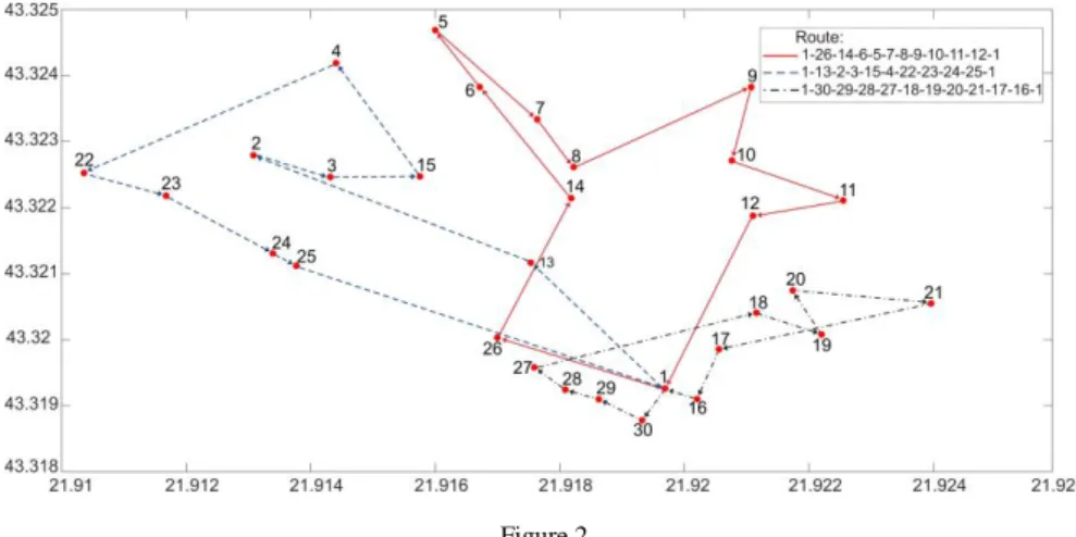
The application of the IHSA also led to an improvement in the initial solution through the use of the recommended algorithm parameters. This application yielded three routes with the total route duration time of 244.24 min. Figure 2 shows the appearance of the transport network routes.

Figure 2

Graphic representation of the VRPSD routes obtained by the IHS algorithm

Conclusion

A combination of the constructive heuristic and metaheuristic algorithms was applied to optimize the movement routes of municipal waste collection vehicles for the observed transport network. The improvements introduced by thus designed routes in comparison with the existing routes used by the PUC “Mediana-Niš”

vehicles relate to the reduction in the total travel distance and the reduction in the total working hours of the operator and vehicle that collect municipal waste. The

average route length of the PUC “Mediana-Niš” municipal waste collection vehicles for the observed transport network is 65.33 km/day, while the route length for the same transport network obtained by the VRPSD optimization is 59.82 km/day [21].

These results show that the application of the proposed solution can lead to a reduction in the mechanization fuel costs of up to 10%.

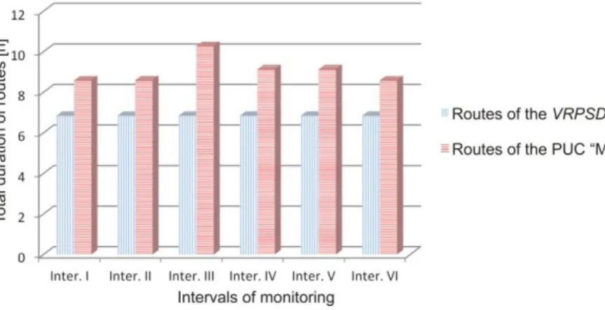
Figure 3 shows the relation between the consumed time per day for the routes obtained by solving the VRPSD and the routes currently used by the municipal waste collection vehicles of the PUC “Mediana-Niš”. The graph shows that the VRPSD routes are shorter in comparison with the routes used by the PUC

“Mediana-Niš” vehicles. The average route duration time obtained by solving the VRPSD is 6.84 h/day, while the average route duration time of the PUC

“Mediana-Niš” vehicles is 9.05 h/day.

Figure 3

Graphic representation of the total duration of the VRPSD routes and the existing PUC “Mediana-Niš”

routes

All this shows that the vehicle routes for municipal waste collection in the observed transport network are optimized. The developed VRPSD model represents a real model, bearing in mind that it takes into consideration all of the parameters that could influence the operation of a municipal waste collection vehicle in an urban area. Furthermore, the developed methodology possesses a universal character and it can be applied to any urban area. Results presented are compatible with current trend of inclusion of Industry 4.0 technologies in waste collection routing [23], which involves cyber-physical systems paradigm, Internet- of-things, big data, cloud computing and other technologies, which all together represents important research direction beyond our results. Also, optimization techniques used in this study are selected as most suitable and providing good resuts from a much larger set of tested algorithms, so comparative study of suitability of these techniques in considered case is also important prospect for further research.

Acknowledgement

This paper is part of the project TR-35049 implemented at the University of Niš, Faculty of Mechanical Engineering, and supported by the Ministry of Education, Science and Technological Development of the Republic of Serbia.

References

[1] Dantzig, G. B., Ramser, J. H. (1959) The truck dispatching problem, Management science, 6(1), pp. 80-91

[2] Benjamin, A. M. (2011) Metaheuristics for the waste collection vehicle routing problem with time windows, PhD thesis, Department of Mathematical Sciences, Brunel University, London, United Kingdom

[3] Letchford, A. N., Salazar-González, J. J. (2019) The capacitated vehicle routing problem: stronger bounds in pseudo-polynomial time, European Journal of Operational Research, 272(1), pp. 24-31

[4] Laporte, G., Nobert, Y., Desrochers, M., (1985) Optimal routing under capacity and distance restrictions, Operations Research, 33 pp. 1050-1073 [5] Laporte, G. (2018) Vehicle routing with backhauls, Computers and Operations

Research, 91(C), pp. 79-91

[6] Csiszár, S. (2005) Route elimination heuristic for vehicle routing problem with time windows. Acta Polytechnica Hungarica, 2(2), 77-89

[7] Madankumar, S., Rajendran, C. (2018) Mathematical models for green vehicle routing problems with pickup and delivery: A case of semiconductor supply chain, Computers & Operations Research, 89, pp.183-192

[8] Mohamed, M. K., Lanzon, A. (2012) Design and control of novel tri-rotor UAV, IEEE International Conference on Control (CONTROL) UKACC, pp.

304-309

[9] Avci, M., Topaloglu, S. (2016) A hybrid metaheuristic algorithm for heterogeneous vehicle routing problem with simultaneous pickup and delivery, Expert Systems with Applications, 53, pp. 160-171

[10] Marinakis, Y., Iordanidou, G. R., Marinaki, M. (2013) Particle Swarm Optimization for the Vehicle Routing Problem with Stochastic Demands, Applied Soft Computing, 13(4), pp. 1693-1704

[11] Xiangyong, L., Peng, T., Stephen, C. H. L. (2010) Vehicle routing problem with time windows and stochastic travel and service times, International Journal Production Economics, 125, pp. 137-145

[12] Bautista, J., Fernadez, E., Pereira, J. (2008) Solving an urban waste collection problem using ants heuristics. Computers & Operations Research, 35(9), pp.

3020-3033

[13] Vera, H., Karl F, D., Richard F, R., Stefan, R. (2013) A heuristic solution method for node routing based solid waste collection problems. Journal of Heuristics, 19,(2), pp. 129-156

[14] Radiša, R., Dučić, N., Manasijević, S., Marković, N., Ćojbašić, Ž. (2017) Casting improvement based on metaheuristic optimization and numerical simulation. Facta Universitatis, Series: Mechanical Engineering, 15(3), 397- 411

[15] Marković, D. (2018) Development of a logistic model for municipal waste management by applying heuristic methods, PhD Thesis, University of Niš, Serbia

[16] Tao, Z., Chaovalitwongse, W. A., Yuejie, Y. (2012) Scater search for the stohastic travel-time vehicle routing problem with simultaneous pick-ups and delivers. Computers & Operations Research, 39, pp. 2277-2290

[17] Coutinho-Rodrigues, J., Tralhão, L., Alçada-Almeida, L. (2012) A bi- objective modeling approach applied to an urban semi-desirable facility location problem. European Journal of Operational Research, 223(1), 203- 213

[18] Tomić, V., Marinković, D., Marković, D. (2014) The selection of logistic centers location using multi-criteria comparison: case study of the Balkan Peninsula. Acta Polytechnica Hungarica, 11(10), 97-113

[19] Ghiani, G., Laganà, D., Manni, E., Triki, C. (2012) Capacitated location of collection sites in an urban waste management system. Waste management, 32(7), 1291-1296

[20] PUC “Mediana-Niš”, 2017, Public utilities company “Mediana-Niš”, Serbia [21] Marković, D., Petrović, G., Ćojbašić, Ž., Stanković A. (2017) The vehicle

routing problem with stochastic demands in an urban area –a case study. Facta

Universitatis, Series: Mechanical Engineering,

DOI:10.22190/FUME190318021M

[22] Marković, D., Madić, M., Petrović, G. (2012) Assessing the performance of improved harmony search algorithm (IHSA) for the optimization of unconstrained functions using Taguchi experimental. Scientific Research and Essays, 7(12), pp. 1312-1318

[23] Bányai, T., Tamás, P., Illés, B., Stankevičiūtė, Ž., & Bányai, Á. (2019) Optimization of Municipal Waste Collection Routing: Impact of Industry 4.0 Technologies on Environmental Awareness and Sustainability.

International journal of environmental research and public health, 16(4), pp.

634