Two-Phase Heuristic for the Vehicle Routing Problem with Time Windows
Sándor Csiszár
Institute of Microelectronics and Technology
Kálmán Kandó Faculty of Electrical Engineering, Budapest Tech Tavaszmező u. 17, H-1084 Budapest, Hungary
E-mail: csiszar.sandor@kvk.bmf.hu
Abstract: The subject of the paper is a complete solution for the vehicle routing problem with time windows, an industrial realization of an NP hard combinatorial optimization problem. The primary objective –the minimization of the number of routes- is aimed in the first phase, the secondary objective –the travel distance minimization- is going to be realized in the second phase by tabu search. The initial route construction applies a probability density function for seed selection. Guided Route Elimination procedure was also developed. The solution was tested on the Solomon Problem Set and seems to be very compeitive with the best heuristics published in the latest years (2003-2005).
Keywords: Metaheuristics; Vehicle routing problem; Time windows; Tabu search;
Combinatorial optimization
1 Introduction, Problem Definition
At transportation an important question is -next to the in time delivery- the cost of the service. The lowest number of routes is primarily important because it determines the number of vehicles applied. The second priority is the minima of the total travel distance. There are studies where the secondary objective is the minimum schedule time when quick and in time service is more important than the travel distance. The VRP has a large literature, so here only a short introduction is given. Let G = {V, E} be a graph and V = {v0, v1, ... , vn} a set of vertices representing the customers around a depot, where vertex v0 denotes the depot. A route is a closed tour, starting from and entering the depot: {v0, ..., vi, vj, ..., v0}. The cost of a tour is:Ct =
∑
(route)di,j, where i and j are consecutive customers on the route and di,j∈E. The objectives of the solution are to determine the lowest number of routes -or number of vehicles (Nv)- and the lowest cost (total travel distance, C=∑(s)Ct , where (s) is the actual solution), providedthat each customer can be visited only once. The specific problem instances are given by the the number of customers, their demand, delivery time windows, service time and customer coordinates. The vehicle capacities are identical and given for each problem type. The distances between the customers are the Euclidian distances. The service must be started within the given time window, the vehicle travel time constraint is determined by time window of the depot. (The violation of the constraints is not allowed in a feasible solution.)
Mathematical formulation of VRP with Time Windows (VRPTW) can be found in the relevant literature [14]. Although there are exact methods [10] [11], their application is limited because the computation time is excessively increasing with the number of customers. The solution of this problem has double objective, and it implies the real advantage of the two-phase solution. The chance of one phase heuristics for route elimination is quite low. The explanation is: neighbourhood solutions don’t represent so significant changes that would be required for eliminating quite long routes. In addition the routes become ever longer as the search is progressing. The other reason is, the lowest cost is -sometimes- not at the lowest number of routes. If we analyse the performance of the tabu search (TS) we must admit that despite it is one of the most successful metaheuristics it has difficulties in special cases when the route elimination goes together with cost increment. The objective function of the TS is usually designed for finding cheaper solutions. We can change the objective function and the length of the tabu-list but it is difficult for a pure TS algorithm to get out from ‘deep valleys’ so the search is basically guided by the secondary objective. In the route elimination respect -although it is the primary objective- the pure TS loses to other –lately developed- hybrid metaheuristics [2].
The remaining part of the paper is structured as follows. Section 2 is about the initial route construction, Section 3 describes the guided route elimination, Section 4 is the second phase by tabu search, and finally Section 5 is about the conclusion, computational results and future plans.
Notations used in the article:
C : Total cost of the solution or total travel distance (TTD), TCi : Time constraint factor of customer i,
TC : Average time constraint of the problem, Nv : Number of vehicles (number of routes), Nr : Number of customers on the actual route, ItNo : Actual iteration number,
tli : Latest time to start service at customer i.
tei : Earliest time to start service at customer i.
ti : Actual arrival time at customer i, ri : Customer distance from depot,
rmax : Depot distance of the farthest customer, rij : Distance between customer i and j,
i'
r : Relative customer distance from depot,
ns : Initial seed number for parallel route construction, n : Total number of customers,
n0 : Number of customers in the seed selection zone;
twb , twa : waiting time before and after the insertion, α, λ, ω: Cost function parameters.
2 Initial Solution
At the design of the Initial Route Construction (IRC) the main objective was to obtain quick and good quality solutions (first of all in respect of the number of routes) within reasonable computation time. The intention was to design a heuristic that maps the most important considerations of a human being. These are as follows: (It is noted that nodes and customers are used as synonyms in the article.)
a) distance from the depot,
b) waiting time before and after the insertion,
c) distance between customers affected in the insertion,
d) savings (cost difference realized by the actual solution, compared to serving the single customer by another extra vehicle),
e) route building in both directions, f) time window of the given customer,
g) demand of customers in order to fill the trucks optimally -especially at those problems, where the vehicle capacity represents a strict constraint, h) taking care of not leaving a single customer alone unrouted (otherwise an
expensive extra route should be devoted to serving that), i) parallel route construction,
j) step back if the partial solution seems to be unfavourable.
2.1 The Objective Function
In the literature a known objective function is used for insertion heuristics (Eq. 1) calculating the cost if node k is inserted between node i and node j. Items (a,) (b,)
(c,) (d,) (e,) are also considered in Eq. 1. Item (f,) has an important role in the insertion sequence, because the narrower the time window of a certain customer the more difficult it is to insert this customer into a route, so we have to give preference to customers with narrow time window. The time constraint factor (TCi) was introduced in order to realize this preference in the mathematical formulas:TCi =(tli−tei)/(tl0−te0). The average time constraint factor is also needed for dimensionless description:TC =1/n∑TCi . The new objective function is formulated in Eq. 2, where ω is used for getting a realistic weighting in order to moderate the drastic time constraint effect.
k wb wa ij
kj ik
k r r r t t r
c =α( + − )+(1−α)( − )+λ (1)
[
ik kj ij wa wb]
kk
k TC TC r r r t t r
c =( / )ωα( + − )+(1−α)( − ) +λ (2)
Computational tests show thatω=[0.35L0.7]gives the best results. Customers - having narrower time windows- seems to be cheaper for the algorithm, this way we can stimulate them. This change in Eq. 1 made a perceptible improvement in the results: 1.57% improvement in the number of routes. It worth mentioning that Eq. 2 was tested with reduced time constraint factor: TCi =(tli−tact)/(tl0−te0), where tact is the actual possible time of starting service at the selected customer. It seems to be rational to consider only that part of the time window that is available for service in the actual situation. Even if the customer has a wide time window and it is unrouted at a certain situation, it may be critical for the service if the remained available time for service is short. With the application of the idea no further improvement could be detected on the sample problems.
2.2 Seed Selection for Route Initialization
The essence of this concept is the following: seed points are selected from a cirkular-ring zone (r'>rsb), those customers that are far from the depot or have a low value of TC factor are favoured as seed points. The applied probability function for seed selection is Eq. 3. A detailed description of the probability based seed selection can be found in [6].
⎪⎩
⎪⎨
⎧
≤
≥
>
≥
<
=
) 4 . 0 ( ) ' ( ) / ( ) / ' (
) 4 . 0 ( ) ' ( )
/ ' (
) ' ( 0
i sb
i b
i a
sb i
i sb
i a
sb i
sb i i
TC and r r if TC TC r r
TC and r r if r
r
r r if
p (3)
Let the relative depot distance be:ri'=ri/rmax, where rmax is the distance of the farthest customer from the depot. It seems to be rational to define a minimum radius around the depot, within that radius seeds are not selected. Let’s define this radius as a relative seed border: rsb. Usually rsb =0.5 is sufficient for this but in
special cases it is necessary to reduce this value according to have sufficient number of customers -min{2Nv, 0.35n}- in the circular-ing zone. Reduce the actual value of rsb until the above condition is satisfied.
The parameters of Eq. 2 are α, λ¸ and ω. The following parameter combinations [1] resulted 42 initial solutions:α=[0.5L1]in 0.1 steps, λ =[0.5L1.7]in 0.2 steps and ω =0.5.
2.3 IRC Algorithm
(TCi and TC are calculated after data retrieve);
1. Set α from the interval[0.5L1]and λ from[0.5L1.7]; 2. Set rsb = 0.5 (for the seed border);
3. Preliminary route construction;
(to find out the preliminary number of routes: Nvp);
4. Count the number of customers in the seed selection zone (no);
5. while n0<min(2Nvp,0.35n) do
sb
sb r
r :=0.975⋅ ; Count n0; 6. end while;
7. Set R:=O/ (set of routed nodes);
8. Set U:={ui} i=1,2,K,n (set of unrouted nodes);
9. Set S (set of unrouted nodes in the seed selection zone);
10. Repeat
11. Set p:=−1; r:=3⋅rmax; 12. for (∀i∈R) and (∀j∈S) do 13. If rij <r then
14. p:= j; r:=rij; 15. end if;
16. end for;
17. if r<1.5⋅r then v:= p (it means that a customer remained unrouted close to the full route in the seed zone, so it is selected) 18. else
19. if (p:=−1) then
20. Let v:=i|r0i >r0j,∀(i,j)∈U (there are no unrouted customers in seed zone, so the farthest one is selected)
21. else
22. v is selected by Eq. 3 23. end if;
24. end if;
25. R←{v}; U:=U−{v};
26. If rv ≥rsb then S:=S−{v} end if;
27. Initialize a route k: 0 - v - 0;
28. v:=Select node for insertion using Eq. 2;
29. while (v≠O/ ) do
30. Insert node v into route k;
31. R←{v}; U:=U−{v};
32. If rv ≥rsb then S:=S−{v} end if;
33. v:=Select node for insertion using Eq. 2;
34. end while;
35. Until (U ≠O/ )
The described algorithm was embedded in a cycle to compute the 42 initial solutions, then the best one (with the lowest number of routes) was selected for further processing. 10 computational runs were made on each of the 56 Solomon problems and compared to the best results found by metaheuristics. The average of the ever found best number of routes is 7.23 the same figure of IRC was 7.80.
The result of the initial route construction algorithm is good also in the best one comparison.
3 First Phase
An exercise was made in the study how a general attribute of the problem can guide the search and how successful it is. This attribute is the total cost of the solution.
3.1 The Route Elimination
The developed route elimination algorithm is a recursive procedure that applies the in depth-first search. Depth of the search tree (6L8) depends on the average time constraint (TC), because the wider the time windows are the higher the complexity of the search is.
The most promising route has to be selected first for elimination. Three types of route selection methods are used. The first method is based on the number of nodes on the route (the shorter routes are preferred). The second one takes also the insertion frequency of the nodes into account. It can not be used at the beginning of the search and 65-35% weighting is applied between the number of customers on the route and the insertion frequency by the following equation:
∑
⋅
− +
⋅
=min[0.65N N /n 0.35(1 N /(ItNo N ) ins)]
selCrit r v v r (4)
The third route selection procedure based on the route selection frequency. This latest one prefers those routes that are selected rarely. The route selection is controlled by the block management unit. The successful insertion frequency and the number of route elimination trials per route are collected in a database. These data are used for two purposes: route selection for elimination, insertion sequence of nodes. If the remained nodes after trial have a favourable insertion statistics it means the chance for success is higher at the post search.
The in depth-first search is executed within given cost limits, otherwise expensive insertions and changes cause dramatic total travel distance increment. The only exception is the last node, provided that all the previous insertions were successful -in this case the cost limit is not considered. If a certain route is selected for elimination all its nodes are tried to be inserted onto other routes. The first task is to determine the insertion sequence of the customers on the selected route. As the computational trials show it is an important part of the route elimination algorithm.
Insertions are tried with reasonable cost limit:
[
2L2.6]
⋅r. The purpose of this limit is to avoid drastic cost increment that would hinder further insertions. If the insertion fails then 3-Opt insertions are tried provided the time windows are wide.A learning process is embedded in the route construction phase that counts the success of the 3-Opt intra route changes and these data are used for making decision about the 3-Opt insertions. If the success ratio reaches a certain percent the 3-Opt internal reordering is used before insertions otherwise not. If 3-Opt insertions fail intelligent reordering is tried [1].
Until no unsuccessful insertion occurs, in case of failure a repair procedure is activated after a couple of cost reduction steps. First the graph has to be modified by the TS algorithm in order to reduce the total travel distance. On both sides around the unsuccessfully inserted customer all the routes have to be identified in two times 40° sector (or in a user given angular domain). Try to combine these routes every feasible way (2-Opt) and at each route combination try the search again.
After the route elimination if a reasonable number of customers remains unrouted and their time constraint factors and depot distances satisfy certain criteria a Post Search is taking place. The evaluation of the remained nodes is made by an
algorithm that considers the depot distance, TC factors and also the insertion data provided the number of iterations is higher than a defined value (5⋅Nv).
If the route elimination was not successful and only a few customers –less then Nv
n/ ) 3 . 0 2 . 0
( L - remained unrouted it seems to be rational to fill the route up as much as possible in order to draw off customers from other routes and at the same time to increase diversification. The filling up is done by varying the parameters (α, λ, ω) in Eq. 2.
3.2 Concept of Guided Route Elimination (GRE)
GRE is the core procedure of the developed route elimination. During the route elimination a list is used to prevent evolution of circles in customer exchange. It was observed that a number of nodes don’t move from their place during the route elimination. That means the search is limited to a certain neighbourhood.
Obviously it comes from the neighbourhood graph definition that only a limited subset of solutions can be reached from a given solution. The main idea was to enforce the unmoved nodes to a certain extent. It is well known at the tabu search if no cheaper solution is found in the neighbourhood -provided the tabu list is not hurt, in this case those nodes are penalized which move frequently. The penalization is made by the following equation: dk' =dk −const⋅fm, where fm is the move frequency registered in a database. The value of the constant
[
5L10]
has no effect on the search. In this case the modified cost (dk') is used for selection instead of the real cost (dk) and the Tabu Search finds the move of the least penalized customers cheaper and prefers their move to reveal new regions in the solution space.
The essence of the GRE concept is: not only the moves enforced by tabu search but those evoked by the ‘in depth first search’ are counted and added to the move frequency. This way the unmoved nodes are forced. In order to moderate this effect the cost increment has to be controlled. The Search management checks regularly the total cost and compares it to the initial cost. If the relative cost increment is higher than the user defined value
[
1.1L1.2]
the customer move frequency data of TS are readjusted to the starting value (100). For this reason the algorithm is divided into search blocks. The starting value was defined to 100 because it gave a realistic block cycle number(45L50)and the move ratio between the TS and the GRE is about80/20%.3.3 A Route Elimination Cycle
1. Let p1 = Random(100) be; (start of the route selection)
2. if (p1 < 30) then Select one of the rarely tried routes (based on statistics) 3. else
4. if (no statistical data available) then
5. Find the route with the lowest number of customers;
6. else
7. Selection based on statistical data;
8. end if ;
9. end if ; (end of the route selection) 10. firstFail:=False;
11. costContrCount := 0;
12. Repeat
13. Select customer for insertion (using MSA);
14. InsOK:=False;
15. if Recursive insertion is successful then InsOK:=True end if;
16. if Not InsOK then
17. if 3-Opt Recursive insertion is successful then InsOK:=True end if;
18. end if;
19. if Not InsOK then
20. if Intelligent Reordering recursion is successful then InsOK:=True end if;
21. end if;
22. if Not InsOK and Not firstFail then 23. Cost reduction cycles;
24. costContrCount := 0;
25. if Not Repair algorithm (recursion) is successful then firstFail:=True end if;
26. else
27. Inc(costContrCount);
28. end if;
29 If (costContrCount > allowedNo) then 30 Cost control cycles;
31 costContrCount := 0;
32 end if;
(The allowedNo depends on the initial number of customers on the route.)
33. Until No more nodes is found;
34. If (No. of unrouted customers>0) then Post Search end if;
3.4 Multi Strategy Application
This is a successful tool used several time in the solution. Route selection for elimination, the route elimination cycle and the node insertion sequence combines several strategies. According to the experiences an intelligent strategy works well at a problem instance and fails at the other. Certain strength can be the weakness at another problem type. The question is: how can we maximize the exploitation of the good strategies? The following method is proposed:
- Find out promising strategies.
- Decide on the priority order (or probability values) and the application rules.
- Use the application rules and probability functions for the application of strategies.
- Change the probability values during the search according to the success ratio (optional learning).
4 Second Phase: Tabu Search
In the second phase of the developed metaheuristic the same tabu search was applied for finding cheaper solution as it was used for controlling the TTD at the guided route elimination. The basis of this TS solution was the reactive tabu search [3] with some differences, first of all in the used operator set and the tabu list. The extinct arcs are stored on the tabu list instead of route and node identifiers. This is less restrictive, although in case of arc (i-j) on tabu the re- creation of this arc is not allowed, but if the route identifier and the relevant node is stored on tabu it is possible on another route.
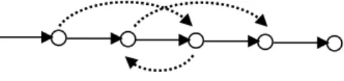
The used insertion and the interchange operators are always evaluated using global best (GB) strategy. If no cheaper solution is found the next operators is used in the following order: intra route 3-Opt (Fig. 1), interchange-21 (two nodes from one route and one from the other are swapped if it is feasible), interchange- 22, interchange-32. These operators slow down the procedure but gives better results. The tabu list tenure is managed in the interval of
[
6L12]
. At the beginning of the second search phase the tabu list is initialized with an empty list and the best solution is taken from the first phase. The aspiration criteria is applied, if the found solution is better than the global best the tabu list is neglected. In case of a significant cost or waiting time reduction intensification ismade realizing that by an intensification list. A maximum of 3000 iteration steps was adjusted.
Figure 1 Intra route 3-Opt changes
5 Computational Results, Conclusion, and Future Plans
The presented two-phase algorithm (HGRE) is tailored to middle size VRP with Time Windows. A summary of its main contributions are as follows:
1 The objective function (Eq. 2) qualifies the unrouted nodes for insertion taking also the width of the time windows into account (Eq. 1). A similar concept was applied at the seed selection for route initialization [6].
2 It was found the continuous control of Total Travel Distance (TTD) aids route elimination. A Guided Route Elimination concept (GRE) was realized to explore the solution space as much as possible.
3 A learning process was built into the initial route construction phase (the success ratio of 3-Opt intra route changes is collected and calculated) to use that at the route elimination in order to save computation time. If the success ratio reaches a given limit the 3-Opt insertions are tried otherwise not.
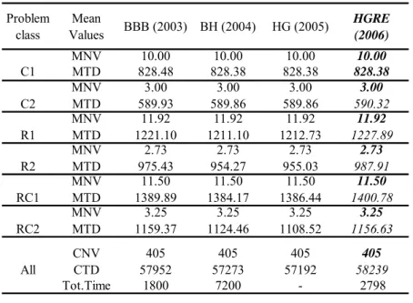
The computer program for the developed two-phase algorithm was written on Delphi platform by dynamic memory programming and was tested on the Solomon Problem Set on 1.7 GHz computer. The user surface of the developed computer probram can be seen on Figure 2. A maximum pre-adjusted search time was 30 minutes. At the initial route construction and at the route filling up α, λ, ω were varied in order to generate initial solutions, the minimum tabu tenure was 6 the maximum was 12. The cost limit used at the in depth-first search was:rik +rkj ≤2.6r. It is quite difficult to find perfect comparison, first because of the continuous improvement of the computer platforms, processors and RAM capacities, secondly because of the differences in the used parameters, the optimization criteria and the programming languages. The performance of the developed HGRE seems to be very competitive with the lately published best algorithms found in the literature (Table 1).
Problem class
Mean
Values BBB (2003) BH (2004) HG (2005) HGRE (2006)
MNV 10.00 10.00 10.00 10.00
C1 MTD 828.48 828.38 828.38 828.38
MNV 3.00 3.00 3.00 3.00
C2 MTD 589.93 589.86 589.86 590.32
MNV 11.92 11.92 11.92 11.92
R1 MTD 1221.10 1211.10 1212.73 1227.89
MNV 2.73 2.73 2.73 2.73
R2 MTD 975.43 954.27 955.03 987.91
MNV 11.50 11.50 11.50 11.50
RC1 MTD 1389.89 1384.17 1386.44 1400.78
MNV 3.25 3.25 3.25 3.25
RC2 MTD 1159.37 1124.46 1108.52 1156.63
CNV 405 405 405 405
All CTD 57952 57273 57192 58239
Tot.Time 1800 7200 - 2798
Table 1
Comparison on Solomon benchmark problems. BBB: Berger et al. [16], BH: Bent and Van Hentenryck [17], HG: Homberger and Gehring [9]
Figure 2 HGRE application
The best results were selected from a series of 10 independent runs per problem instance then the mean number of vehicles (MNV), mean travel distance (MTD) and the mean computation time per problem type (MCT) were calculated.
Additionally the cumulated number of vehicles (CNV) and the cumulated travel distance (CTD) are reported. Bold letters are used if the found value is the best one or equals to the best known result.
It is important to analyse the time requirement of the HGRE algorithm. The time percentage of the initial route construction is 5.5%, that of the route elimination is 15.5% and the tabu search is the most significant time consuming part of the algorithm with 79%. The route elimination is quite quick, although there are several ‘heavy’ problems for the algorithm, especially where the best number of routes is less then 4, consequently 25-30 customer nodes have to be inserted.
For further development a possible way to use a simpler cost control algorithm in order to further reduce the computation time. For large problem instances more sophisticated intelligence is needed in order to decide about the application of the time consuming search. At the neighbourhood structure the Global Best strategy has to be replaced by First Best or investigate only a certain part of the neighbourhood to get a reasonable computational time at large problems.
Acknowledgement
The author whish to thank Prof. Dr. László Monostori (Budapest University of Technology and Economics and Deputy Director of Computer and Automation Research Institute of the Hungarian Academy of Sciences) and Dr. Tamás Kis (Computer and Automation Research Institute of the Hungarian Academy of Sciences) for their help and useful advices, Dr. Péter Turmezei (Head of Department of Microelectronics and Technology, Budapest Tech, Hungary) for his support.
References
[1] O. Bräysy, A Reactive Variable Neighbourhood Search for the Vehicle- Routing Problem with Time Windows, Informs Journal on Computing 15 (2003) pp. 347-368
[2] O. Bräysy, M. Gendreau, Tabu Search Heuristics for the Vehicle Routing Problem with Time Windows, Sociedad de Estadística e Investigación Operativa, Madrid, Spain (December. 2002)
[3] W. C. Chiang, R. A. Russell, A Reactive Tabu Search Metaheuristic for the Vehicle Routing Problem with Time Windows, Journal on Computing 9 (1997) pp. 417-30
[4] W. C. Chiang, R. A. Russell, Simulated Annealing Metaheuristic for the Vehicle Routing Problem with Time Windows, Annals of Operation Research 63 (1996) pp. 3-27
[5] G. Clarke, J. W. Wright, Scheduling of Vehicles from a Central Depot to a Number of Delivery Point, Operation Research 12 (1964) pp. 568-581 [6] S. Csiszár, Sequential and Parallel Route Construction based on Probability
Functions for Vehicle Routing Problem with Time Windows, 5th International Conference IN-TECH-ED (2005) pp. 379-388
[7] Glover F. Tabu Search, Part I. ORSA J. Computing, 1 (1989) pp. 190-206 [8] Glover F. Tabu Search, Part II. ORSA J. Computing, 2 (1990) pp. 4-32 [9] J. Homberger, H. Gehring, A Two-Phase Hybrid Metaheuristic for the
Vehicle Routing Problem with Time Windows, European Journal of Operation Research, 162 (2005). pp. 220-238
[10] G. Laporte, The Vehicle Routing Problem: An Overview of Exact and Approximate Algorithms, European Journal of Operation Research 59 (1992) pp. 345-58
[11] G. Laporte, Y. Nobert, Exact Algorithms for the Vehicle Routing Problem, In S.Martello, G. Laporte, M. Minoux, C. Riberio, editors, Surveys in Combinatorial Optimization, Amsterdam North-Holland (1987) pp. 147-84 [12] M. M. Solomon, Algorithm for the Vehicle Routing and Scheduling
Problem with Time Window Constraints, Operation Research 35 (1987) pp.
254-265
[13] E. Taillard, Parallel Iterative Search Methods for Vehicle Routing Problems, Networks 23 (1993) pp. 661-72
[14] S. R. Thangiah, I. H. Osmann T. Sun, Hybrid Genetic Algorithms, Simulated Annealing and Tabu Search Methods for Vehicle Routing Problem with Time Windows, Technical Report UKC/OR94/4, (1995) Institute of Mathematical Statistics, University of Kent, Canterbury, UK [15] A. Van Breedam, A parametric Analysis of Heuristics for the Vehicle
Routing Problem with Side-Constraints, European Journal of Operation Reports 137 (2002) pp. 348-370
[16] J. Berger, M. Barkaoui, O. Bräysy, A Route Hybrid Generic Approach for the Vehicle Routing Problem with Time Windows, INFORMS 2003, 41 (2) [17] R. Bent, PV. Hentenryck, A Two-Stage Hybrid Local Search for the
Vehicle Routing Problem with Time Windows, Transportation Science 2004, 38 pp. 515-530