Route Elimination Heuristic for Vehicle Routing Problem with Time Windows

Route Elimination Heuristic for Vehicle Routing Problem with Time Windows

Sándor Csiszár

Department of Microelectronics and Technology, Budapest Tech Tavaszmező u. 17, H-1084 Budapest, Hungary

csiszar.sandor@kvk.bmf.hu

Abstract: The paper deals with the design of a route elimination (RE) algorithm for the vehicle routing problem with time windows (VRPTW). The problem has two objectives, one of them is the minimal number of routes the other is the minimal cost. To cope with these objectives effectively two-phase solutions are often suggested in the relevant literature. In the first phase the main focus is the route elimination, in the second one it is the cost reduction. The algorithm described here is a part of a complete VRPWT study. The method was developed by studying the graph behaviour during the route elimination. For this purpose a model -called “Magic Bricks” was developed. The computation results on the Solomon problem set show that the developed algorithm is competitive with the best ones.

Keywords: Vehicle routing problem, Time windows, Tabu search, Transportation

1 Introduction, Problem Definition

The Vehicle Routing Problem (VRP) has a rich literature, so in this paper only a short introduction of the topic is given. VRP is well known combinatorial NP hard problem having several industrial realizations: VRP with time windows, multi- depot, split delivery or other similar problems such as Travelling Salesman Problem, Bin packing, or Job-shop scheduling. Whether the subject of transportation is the raw-material supply to manufacturers or distribution of end products to vendors a vitally important question – next to the in time delivery and quality of the transportation – is the cost of the logistics service. To solve these problems effectively good logistics management is required including vehicle routing optimization. The lowest number of routes is primarily important because it determines the numbers of vehicles applied, consequently influences the investment and fix cost of the company. The second priority is the minima of the total travel distance. There are studies where the second objective is the minimum schedule time when quick and in time service is more important then the travel

distance. Exact mathematical formulation of VRP can be found in [1]. Problem characteristics are as follows:

• the number of customers, their demand, delivery time windows, service time, customer positions – coordinates – and vehicle capacities are given,

• distances between customers and depot are determined by the Euclidean distances,

• all vehicles start from and arrives at the depot,

• all customers can be visited only once,

• the capacity of vehicles is maximized and uniform and must not be violated,

• the service must be started within the given time window of the customer,

• vehicle travel time constraint is given by the depot time window.

As we know, the application of exact methods in the VRP problem solving is quite limited because of the combinatorial “explosion”. During the decades different successful metaheuristics have been developed, for instance Simulated Annealing, Evolutionary Algorithms, and Tabu Search (TS) etc. If we analyse the TS we must admit that despite its indisputable success it has problems in special cases when the route elimination goes together with considerable cost increment. Normally the object function of the TS is designed for finding cheaper solutions. Depending on the length of the tabu list the algorithm is able to reveal new regions. We can in the meantime change the object function and the length of the tabu-list but despite of these techniques it is difficult for the pure TS algorithm to get out from “deep valleys”, so the chance for eliminating a route is quite limited and the search is basically guided by the second priority objective. This topic is detailed in [2]. To leave such kind of deep valleys we have to find effective oscillation – sometimes it is called diversification – methods. In the route elimination respect – although it is the primary objective – the pure TS loses to other – lately developed – metaheuristics first of all hybrid metaheuristics [3]. The purpose of this part of the research and this article is to develop an effective route elimination phase.

The remaining part of the paper is structured as follows. Section 2 describes the

“Magic Bricks” model and its consequences, Section 3 and 4 explains the developed route elimination procedure while Section 5 is about the computational results on route reduction and finally Section 6 is about experiments conclusions and future plans.

2 The “Magic Bricks” (MB) Model

If we want to study the features of the graph during the search we have to find an appropriate model. The graph itself is not suitable for that because all the

information about the graph is in the nodes and we know that it is impossible or at least not worthy– according to our present knowledge and computers – to reveal all the relationships within the nodes if the number of nodes is above 50. Suppose that we have an initial solution. Let the width of a brick the distance – cost – between two nodes on any route and the waiting time is the gap between the bricks. Similarly a single route can be considered a row of bricks in the wall and the whole number of routes would create a wall. Now the objective of VRP can be redrafted: rebuild the wall to get primarily smaller wall – with fewer routes – and secondly try to reduce the length of the brick-rows. We can easily recognize the unique behaviour of this wall, because if we swap any two bricks in the wall each of them changes its width and maybe the following gaps as well. Moreover, not only the two bricks but their predecessors in the rows change similarly, because their neighbours are changed. So swapping two bricks at least four brick widths will change and in bad situation many gaps are affected. From this respect this wall is exactly as complicated as the graph itself, but if we think of the route elimination we can identify its requirements more clearly. If we select a row for elimination:

a) the bricks have to be inserted into the gaps or make series of changes to find an appropriate place for a certain brick,

b) if possible move certain bricks forward or backward (effective in case of wide time windows).

2.1 Consequences of the Model

The point (a) can be satisfied easier if the bricks are narrower – consequently the gaps are wider – that means the chance for successful insertion from a lower cost graph state is better. It must be noted that in case of wide time windows the total waiting time is usually low and the mentioned effect is not significant. This recognition does not mean that from a local minimum it is easy to eliminate a route – the low cost is not a sufficient condition. It means only if we could wander many low cost solutions we could increase the chance of eliminating a route.

Based on this idea a new route elimination (RE) procedure was developed where a continuous cost control is applied. It must be emphasized that owing to the continuous cost control the search is inclinable to clog, that is why a fundamental question is how to ensure the a continuous diversification and the cost control parallel. As far as point (b) is concerned, it is realistic in case of wide time windows. This seemingly increases the chance for the route elimination and it is true if the elimination can be achieved from many graph states (solutions), but at the same time the wide time windows are increasing the complexity of the search.

The success depends on which of the above mentioned effects is stronger.

2.2 Checking the Model in Practice

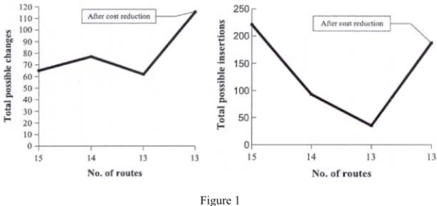
Many computation trials were made to check this model on the Solomon problems, although trials were possible only on those problem instances where the initial number of routes were more then the ever found best one. Explanation below supports the concept. Figure 1 shows how the “flexibility” of the graph is changing during the route elimination and increasing after cost reduction. On the vertical axis for instance the numbers of possible insertions are indicated. These numbers can be obtained the following way: select two adjacent nodes and try all possible insertions excluded the selected one and the depot. Summarize these numbers for each possible pairs on the routes. The charts show a strong increment after the cost reduction especially in the insertion numbers.

Table 1 shows the formation of the route elimination data with and without cost reduction based on 25 cycles for each.

Figure 1

Average insertions and changes on R103 versus number of routes

25 search cycles were made in each case. From low cost solution also the successful ratio was higher and the number of necessary cycles was lower. The computation trials supported the idea to try this concept at the design of a new route elimination algorithm. At the application we must bear in mind two things.

One of them is the extra time needs for the cost control the other one is the earlier mentioned clogging problem – or to avoid that a careful diversification is needed.

Notations used in the following part of the article:

rmax: Depot distance of the farthest customer,

ItNo: Actual number of iterations of the route elimination, n: Number of customers,

Nv: Number of vehicles (routes),

Nr: Number of customers on the actual route, C: Total cost,

r

: Average customers distance,

i: Customer identifier, serial number, ri: Depot distance of the customer i, wi: Waiting time at customer i,

Remark: Not explained equations and parameters in the following part of the article derived from computation run experiences.

Normal search After cost reduction

Ratio of success 72% 84%

Necessary cycles 349 296

Table 1

Success ration of route elimination with and without cost reduction

3 Main Features of RE

The solution is based on depth-first search. Depth of the search tree depends on the average time constraint: =

∑

ⁿ=

i TCi

n

TC 1/ ₁ . In this equation the time constraint factor of customer i is: TC_i=

(

t_li−t_ei

) (

/t_l0−t_e0

)

, where t_ei and t_li are the earliest and latest times to start the service at customer i (depot is costumer 0).

• IF

(

^TC≤0.45

)

THEN depth=8

ELSE IF

(

^TC>0.45

)

^and

(

^TC≤0.6

)

THEN depth=7

ELSE depth=6

• Depth-first search is executed within given cost limits, otherwise the expensive insertions and changes increase the total cost, damaging the first condition detailed in the MB model. The only exception is the last customer provided all the previous insertions were successful, in this case the cost limit is not considered.

• Until no unsuccessful insertion happens in case of failure a repair procedure is activated after a couple of cost reduction steps.

• After the route elimination, if a limited number of customers remain unrouted – and their time constraint factor and depot distance satisfy certain criteria – a post search is taking place.

• The whole process is guided by Tabu Search for keeping the total cost down and controlling diversification.

• Successful insertions are registered. These data are used for three purposes:

- route selection for elimination,

- insertion sequence for depth-first search, - diversification made by the TS,

• In case of unsuccessful route elimination, the route – if certain criteria are satisfied – filled up in order to draw away customers from other routes.

4 Detailed Description of the RE Procedure

4.1 Route Selection for Elimination

Three types of root selections are used in the method. The first one selects according to the number of customers on the route (the shorter routes are preferred). The second one takes into account also the insertion frequency of the customers – that can not be used at the beginning of the search – and 65-35%

weighting is applied by the following equation:

( )

[

^{+ −}

_∑ ]

= N N n N ItNoN ins

selCrit min0.65 _{r v}/ 0.351 _v/ _r (1)

In equation (1)

∑

^ins is the total successful insertions of customers on the given route. It is important here to compare only relative quantities such as N_r/N_v. The third one selects by the route selection frequency. This latest one prefers those routes that are selected rarely. The route selection is controlled by the block management unit (Figure 4) and its purpose is to ensure the right balance between the diversification and the selection criteria.

4.2 Route Filling up

If the route elimination was not successful and only a few customers remained unrouted – less then

(

0.2⋅ ⋅⋅0.3

)

n/N_v – then it seems to be rational to fill the route up as much as possible in order to draw off customers from the other routes and at the same time to increase diversification. The filling up is done by combining parameters in the insertion equation:

( ) ( )( )

[

ik ki ij a b

]

k

i r r r w w r

TC

C TC α α λ

ω

+

−

− +

−

⎥⎦ +

⎢⎣ ⎤

=⎡ 1 (2)

Equation (2) is a modified version of cost equation used at insertion heuristics that takes the time window constraint into account. Detailed description can be found in [4].

4.3 Depth-first Search

If a certain route is selected for elimination all the customers are tried to be inserted somewhere onto other routes. Depth-first search was applied because it effectively supports diversification – an important objective as it was stated earlier. The first task is to determine the insertion sequence for the customers on the selected route. At the beginning of the search the following method is used. If there is a customer whose time constraint factor is lower then 0.1 then this customer is selected otherwise a weighting is used considering the depot distance and the TC factor of the customers:

i

i r TC TC

r

selCrit= / _max / (3)

If enough insertion data are available customers with the least successful insertion are tried first. After a costumer has been selected for insertion it is tried first to insert to any possible place with a reasonable cost limit:

(

2⋅ ⋅⋅2.6

)

r. The purpose of this limit is to avoid drastic cost increment that would hinder further insertions.

If this insertion fails try 3-Opt insertions provided the time windows are wide enough. During the initial solution a “learning process is made” the successful intra route 3-Opt insertions are registered and if the success ratio reaches a certain percent the 3-Opt reordering is used – Figure 2 – otherwise not. On Figure 2 a continuous line shows the route before change while a dashed line after that.

Figure 2 Intra route 3-Opt exchanges

If 3-Opt insertions fail try “Intelligent Reordering” suggested by O. Braysy (detailed description can be found in [5]). The main idea of Intelligent Reordering is to try the insertion of customers to an infeasible – previously unsuccessful but promising – place, the insertion cost calculation is made by:

( r

ik

r

ki

r

ij

) ( )( w

a

w

b

) r

k

C = α + − + 1 − α − + λ

(4)

In Equation λ=0, α=0.5. Select the most promising insertion place using Equation (4) where the customer is inserted to. Then the window violated

customer to be looked for. Finally the window violation is resolved by either reordering customers before the window violation or moving customers from the preceding positions to a new position that follows the violated customer. The number of infeasible trials can be decided by the user. If none of the trials of the given customer were successful then compute all the possible swaps of the customer with the earlier mentioned cost limit and try the whole procedure with the replaced customer. The evolution of maybe circles must be blocked by storing all the already executed swaps on the suitable list. The depth of the search gives the number of consecutive swaps as it was described at the main features of the algorithm. If the insertion is unsuccessful and so far no other unsuccessful insertion has been made a repair algorithm is initiated.

4.4 Repair Algorithm

First the graph has to be modified by the TS algorithm in order to reduce the maybe increased cost and to diversify. (Diversification is detailed at the search management.) After that in a user given angle (+/- 40°) at both sides around the unsuccessfully inserted customer all the routes must be identified in two times 40°

sector. Try to combine these routes every possible way according to Figure 3 and at each route combination try the depth-first search again.

Figure 3

Route combination for repair algorithm

4.5 Post Search

If a reasonable number of customers remained unrouted at the end of the depth- first search a post search is executed. A limited number of customers is allowed for the post search:maxCust=2+Trunc(0.1n/N_v). If this criterion is satisfied further investigation is made, because it would not make sense to spend time if there are customers among the remaining ones they have no or very few successful insertions (see data management). At the beginning of the search – no data available – a similar decision is made based on the TC factors and the depot distances of the remained customers. The total cycle number of the post search depends on the outlook for the success:

)]}

, 5 . 0 max(

/ ) min , 3 . 0 max(

[ , 40 min{

maxCycle= Round B_c TC_r r_r

Here Bc is the post search basic cycle time, minTCr is the minimum time constraint factor of the remained customers and r_r is maximum relative depot distance of the

remained customers. Between the post-search cycles there are oscillations, those are identical to that one applied at depth-first search.

4.6 Search Data Management, Data Collection and Processing

During the route elimination procedure a list is used to prevent evolution of circles in customer exchange, additionally the successful insertion frequency and the number of route elimination trials per route are registered and processed later. The insertion frequency is used for three purposes:

• route selection for elimination – already described,

• deciding insertion sequence – also discussed,

• diversification by TS, it is done by the search management.

At the initiation of each search block the customer move frequency data – used by the Tabu Search – are adjusted to 100 as a starting number. In RE procedure TS and the route elimination are sequentially running. If a successful insertion occurs at depth-first search also the customer move frequency of Tabu Search is modified in order to move those customers that are not successful at the insertion. This way the Tabu Search finds their move cheaper and prefers their move to reveal new regions for the depth-first search. As it is known the TS penalises frequently moving customers. This is the basic idea of this route elimination concept. This process must be controlled because after a while the graph would turn into an expensive state that would be disadvantageous for the search – according to the MB model. The Search management checks regularly the total cost and compares it to the initial cost. If the relative cost increment is higher then 1.1 – or the user defined value – then the customer move frequency data of TS are readjusted to 100. The 100 value of the adjusted move frequency must be in accordance with the block cycle to get reasonable cost and diversification ratio. See Figure (4).

5 Computation Results

The worked out RE algorithm is written on Delphi platform by dynamic memory programming and was tested on the Solomon Problem Set on 1.7 GHz computer.

A maximum search time of 30 minutes and fix configuration parameters were used. There are results in the literature with variable configuration parameters also, but at this research it was not applied. Fix parameters were used for the number of cycles in the block management (c1=3) and (c2=5). The cost limit used in the depth-first search and at the cost control cycle was

(

2⋅ ⋅⋅2.6

)

r.

In the literature slightly different comparisons are used. Usually the best result is selected from a given (5 - 18 runs). At this study an average value (10 runs) was applied. In this comparison the algorithm gave the ever found best results in the primary objective and proves to be the best one in the fix configuration parameter category. Similar result was achieved by J. Homberger and H. Gehring with variable parameters.

Figure 4

Block scheme of Route Elimination

In 96% of the total 560 runs the best number of routes was found. The computation time of the whole search process, the initial route construction and the second search phase were registered. The computation time was less then half of the lately developed best solutions. It must be noted that the computation time is the less comparable characteristic of the algorithm because it depends not only on the design of the algorithm itself but on the technical data of the computers (RAM, Processor etc.) and programming language, nevertheless the significant computation time difference can not be explained purely by differences in the

computers.At problem R207 the best result was found in 50% of the runs, at R211 in 40%. At problem R104 and R112 the best result was found in 20% of the runs.

In Table 2-4 the average number of vehicles (MNV) and the best number of vehicles (Best NV) of 10 runs can be seen. The updated best results are available on the website: http://www.sintef.no/static/am/opti/projects/top/vrp/bknown.html

Problem M N V Best M N V Problem M N V Best M N V R101

R102 R103 R104 R105 R106 R107 R108 R109 R110 R111 R112

19 17 13 9.8 14 12 10 9 11 10 10 9.8

19 17 13 9 14 12 10 9 11 10 10 9

R201 R202 R203 R204 R205 R206 R207 R208 R209 R210 R211

-

4 3 3 2.1

3 3 2.5

2 3 3 2.6

-

4 3 3 2 3 3 2 2 3 3 2 -

Average 12.05 11.92 Average 2.84 2.73 Table 2

Computational results, R10X, R20X

Problem M N V Best M N V Problem M N V Best M N V C101

C102 C103 C104 C105 C106 C107 C108 C109

10 10 10 10 10 10 10 10 10

10 10 10 10 10 10 10 10 10

C201 C202 C203 C204 C205 C206 C207 C208

-

3 3 3 3 3 3 3 3 -

3 3 3 3 3 3 3 3 -

Average 10 10 Average 3 3

Table 3

Computational results, C10X, C20X

Problem M N V Best M N V Problem M N V Best M N V RC101

RC102 RC103 RC104 RC105 RC106 RC107 RC108

14 12 11 10 13 11 11 10

14 12 11 10 13 11 11 10

RC201 RC202 RC203 RC204 RC205 RC206 RC207 RC208

4 3 3 3 4 3 3 3

4 3 3 3 4 3 3 3

Average 11.5 11.5 Average 3.25 3.25 Table 4

Computational results, RC10X, RC20X

Conclusion, Future Plans

The worked out method is a part of a research work devoted to VRPTW. The Route Elimination algorithm is based on the described MB model. One of the objectives of the study was to find out if the search can be guided by a general property – total cost – of the graph. The precondition of good realization was to wander the low cost solutions and find one where the depth-first search is effective from. For further development a possible way could be to use a simpler cost control algorithm to further reduce the computation time. For larger number of customers (above 200) more sophisticated intelligence is needed in order to decide on the application of deep search because of its time needs.

Acknowledgement

The author wish to thank Prof. Dr. László Monostori (Budapest University of Technology and Economics and Deputy Director of Computer and Automation Research Institute of the Hungarian Academy of Sciences) and Dr. Tamás Kis (Computer and Automation Research Institute of the Hungarian Academy of Sciences) for their help and useful advices, Dr. Péter Turmezei (Head of Department of Microelectronics and Technology, Budapest Tech, Hungary) for his support.

References

[1] O. Bräysy, W. Dullaert: A fast evolutionary metaheuristic for the vehicle routing problem with time windows, Int. J. AI Tools 12 (2003), pp. 153- 172

[2] J. Homberger, H. Gehring: A two-phase metaheuristic for the vehicle routing problem with time windows, European Journal of Operation Research 162 (2005), pp. 220-228

[3] O. Bräysy and M. Gendreau: Tabu Search Heuristics for the Vehicle Routing Problem with Time Windows. Sociedad de Estadística e Investigatión Operativa, Madrid, Spain (December, 2002)

[4] S. Csiszár: Initial route construction for Vehicle Routing Problem with Time Windows, XXII^nd International Conference “Science in Practice”, Schweinfurt (2005)

[5] O. Bräysy: A reactive variable neighbourhood search for the Vehicle- routing problem with time windows. Informs Journal on Computing 15 (2003), pp. 347-368

[6] A. Van Breedam: A parametric analysis of heuristics for the vehicle routing problem with side-constraints, European Journal of Operation Reports 137 (2002), pp. 348-370

[7] G. Clarke, J. W. Wright: Scheduling of Vehicles from a Central Depot to a number of delivery poing. Operation Research 12 (1964), pp. 568-581

[8] M. M. Solomon: Algorithm for the Vehicle Routing and Scheduling Problem with Time Window Constraints, Operation Research 35 (1987), pp. 254-265

[9] N. Christofides, A. Mingozzi, P. Toth: The vehicle routing problem, Combinatorial optimization, Chichester, Wiley (1979), pp. 315-338

[10] K. Altinkemer, B. Gavish: Parallel savings based heuristic for the delivery problem, Operations Research 39 (1991), pp. 456-469

[11] G. Laporte: The vehicle routing problem: An overview of exact and approximate algorithms, European Journal of Operational Research 59 (1992), pp. 345-358

[12] E. Taillard: Parallel iterative search methods for vehicle routing problems, Networks 23 (1993), pp. 661-672