Power Spectral Density Analysis of Nanowire-Anchored Fluctuating Microbead Reveals a Double Lorentzian Distribution

Article

Power Spectral Density Analysis of Nanowire-Anchored Fluctuating Microbead Reveals a Double

Lorentzian Distribution

Gregor Bánó¹ , Jana Kubacková² , Andrej Hovan¹ , Alena Strejˇcková³ , Gergely T. Iványi⁴,

Gaszton Vizsnyiczai⁵ , Lóránd Kelemen⁵ , Gabriel Žoldák⁶ , Zoltán Tomori² and Denis Horvath^6,*

Citation: Bánó, G.; Kubacková, J.;

Hovan, A.; Strejˇcková, A.; Iványi, G.T.; Vizsnyiczai, G.; Kelemen, L.;

Žoldák, G.; Tomori, Z.; Horvath, D.

Power Spectral Density Analysis of Nanowire-Anchored Fluctuating Microbead Reveals a Double Lorentzian Distribution.Mathematics 2021,9, 1748. https://doi.org/

10.3390/math9151748

Academic Editors: Maria Luminita Scutaru and Junseok Kim

Received: 26 May 2021 Accepted: 21 July 2021 Published: 24 July 2021

Publisher’s Note:MDPI stays neutral with regard to jurisdictional claims in published maps and institutional affil- iations.

Copyright: © 2021 by the authors.

Licensee MDPI, Basel, Switzerland.

This article is an open access article distributed under the terms and conditions of the Creative Commons Attribution (CC BY) license (https://

creativecommons.org/licenses/by/

4.0/).

1 Department of Biophysics, Faculty of Science, P. J. Šafárik University, Jesenná 5, 041 54 Košice, Slovakia;

gregor.bano@upjs.sk (G.B.); andrej.hovan@upjs.sk (A.H.)

2 Institute of Experimental Physics SAS, Department of Biophysics, Watsonova 47, 040 01 Košice, Slovakia;

kubackova@saske.sk (J.K.); tomori@saske.sk (Z.T.)

3 Department of Chemistry, Biochemistry and Biophysics, University of Veterinary Medicine and Pharmacy, Komenského 73, 041 81 Košice, Slovakia; Alena.Strejckova@uvlf.sk

4 Faculty of Science and Informatics, University of Szeged, Dugonics Square 13, 6720 Szeged, Hungary;

itgergo@gmail.com

5 Biological Research Centre, Institute of Biophysics, Eötvös Loránd Research Network (ELKH),

Temesvári krt. 62, 6726 Szeged, Hungary; vizsnyiczai.gaszton@brc.hu (G.V.); kelemen.lorand@brc.hu (L.K.)

6 Center for Interdisciplinary Biosciences, Technology and Innovation Park, P. J. Šafárik University, Jesenná 5, 041 54 Košice, Slovakia; gabriel.zoldak@upjs.sk

* Correspondence: denis.horvath@upjs.sk

Abstract: In this work, we investigate the properties of a stochastic model, in which two coupled degrees of freedom are subordinated to viscous, elastic, and also additive random forces. Our model, which builds on previous progress in Brownian motion theory, is designed to describe water- immersed microparticles connected to a cantilever nanowire prepared by polymerization using two-photon direct laser writing (TPP-DLW). The model focuses on insights into nanowires exhibiting viscoelastic behavior, which defines the specific conditions of the microbead. The nanowire bending is described by a three-parameter linear model. The theoretical model is studied from the point of view of the power spectrum density of Brownian fluctuations. Our approach also focuses on the potential energy equipartition, which determines random forcing parametrization. Analytical calculations are provided that result in a double-Lorentzian power density spectrum with two corner frequencies. The proposed model explained our preliminary experimental findings as a result of the use of regression analysis. Furthermore, an a posteriori form of regression efficiency evaluation was designed and applied to three typical spectral regions. The agreement of respective moments obtained by integration of regressed dependences as well as by summing experimental data was confirmed.

Keywords:nanowire cantilever; stochastic model; double Lorentzian spectrum

1. Introduction

Many of the problems addressed by current nanosciences can be traced back to statis- tical mechanics and the concept of fluctuations. Fundamental problems constantly arise in nanosciences that go beyond conventional findings, complementing the emphasis and motivations of statistical mechanics. Related fields, now broadly referred to as stochastic processes, continue to pose a mathematical challenge.

Stochastic oscillations of anchored mechanical systems immersed in fluidic media or kept in vacuum have attracted significant attention in the past and are important in many ways today. The Brownian motion of a millimeter-sized mirror suspended from a torsion wire was utilized by Kappler back in 1931 to measure the Avogadro constant [1].

The thermal fluctuations of resonant micron-scale mechanical oscillators have been studied

Mathematics2021,9, 1748. https://doi.org/10.3390/math9151748 https://www.mdpi.com/journal/mathematics

extensively, mostly in connection with AFM (atomic force microscopy) cantilevers and MEMS-based (micro- electromechanical) resonators [2–6]. Thermal fluctuations of glass nanofibers and silicon nitride cantilevers have been used to characterize and calibrate such systems for single-molecule force measurements [7,8]. Brownian motion has also been used at a smaller scale in TPM (tethered particle motion) experiments to investigate the properties of linear macromolecules such as DNA [9–11]. In contrast, thermal noise represents the main disturbing and limiting factor in experiments that rely on highly sensitive mechanical and opto-mechanical systems. Examples are inertial sensors [12,13] as well as recently proposed gravitational-wave and dark matter sensors [14–16].

Under certain conditions, system noises and their corresponding statistical quanti- ties can become valuable, measurable features of technological devices and measurement instruments. When a particle immersed in a dissipative medium is simultaneously ex- posed to thermal noise, it reaches an equilibrium state with time, which provides a good possibility to measure statistical properties. Mechanical system fluctuations may also be related to intrinsic damping mechanisms such as internal friction, thermoelastic losses, or losses to the anchor system. Theoretical and experimental interest may then be di- rected toward elucidating the relationships between damping strength and noise. The well-known “fluctuation-dissipation theorem”, which is also used in this work, addresses these general relationships.

The significance of the outputs of the monitored processes is clearly influenced by the equipment parameters and laboratory conditions. As a result, analytical methods differ. The power spectrum of thermal fluctuations can be derived for the case of damped harmonic oscillators [17], which is a good approximation for AFM cantilevers in liquids and gases [3]. The basic oscillator theory was modified by Saulson [17] to account for the thermal noise of mechanical systems, whose losses are dominated by processes occurring inside the material. High external dissipation conditions represent another extreme, which usually happens for low-stiffness micron-scale [7] or even smaller (molecular) systems [18].

When immersed in viscous liquids, these structures operate in a non-resonant, overdamped regime. Interestingly, the same overdamping conditions are present in optical tweezers experiments, where the fluctuation theory was elaborated thoroughly [19,20].

In this work, we investigate the thermal fluctuations of micron-scale viscoelastic mechanical systems submerged in water. In this particular case, as we show below, both the dissipation to the surrounding fluid and the intrinsic damping play an important role.

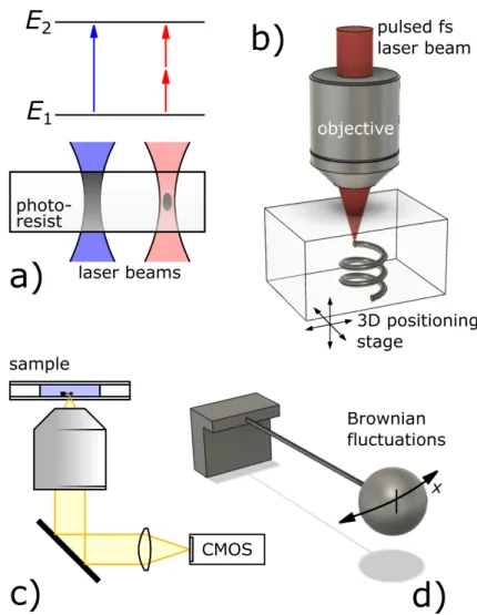
We are interested in the stochastic motion of microbeads attached to cantilevered photopolymer nanowires prepared by two-photon polymerization direct laser writing (TPP-DLW) (see Figure1a,b) [21,22]. The nanowire thickness can be tuned during the fabri- cation process [23]. In the limiting case of thin nanowires, the stochastic thermal forces ex- erted on the microbeads cause clearly detectable Brownian motion behavior (see Figure1c), specifically in the direction perpendicular to the nanowire axis, as depicted in Figure1d).

Moreover, as recently demonstrated, photopolymer nanowires possess viscoelastic ma- terial properties [24,25], which define the specific confinement forces investigated in the present work.

Figure 1.The main steps from sample preparation to measurement. (a) Light-sensitive (photoresist) material exposed to the laser beam. Single photon (left part, in blue) and two-photon (right part, in red) polymerization is depicted separately. (The exceptional spatial resolution can be reached by the two-photon process. The polymerized material is indicated in gray.) (b) The illumination used to produce three-dimensional design in the photoresist volume employing TPP-DLW. (c) Setup for motion detection and data production. The application of a CMOS image sensor, which provides encoded light information about positionx(t)that can be converted into digital data records by particle tracking algorithms. (d) A closer look at the mechanics of Brownian fluctuations under anchoring conditions. The studied fluctuations in the horizontal plane are indicated by the arrows.

Our present work is closely related to the preceding study focused on the bending recovery motion of photopolymer microbead-nanowire systems [25]. A three-parameter linear mechanical model of viscoelastic behavior has been found to provide a good expla- nation of the recovery time-dependence in this study. We aim to use the above theoretical description to include the thermal motion of the microstructure. This can be done analo- gously to other works. The original mechanistic model, which was first developed and validated in [25], can be generalized to reflect random forces. The problem can then be solved using the Fourier transform within the limits of the stochastic steady state in ac- cordance with the experimental setup. The aim is to obtain the corresponding power spectrum and autocorrelation function of Brownian motions of the microstructure analyti- cally. To summarize, our present approach promotes a practical and empirically supported transition from deterministic to stochastic frameworks.

2. Initial Considerations and Model Assumptions

Our main objective is to describe the stochastic motion of viscoelastic microstructures composed of cantilevered nanowires and spherical beads (see Figure 1) immersed in Newtonian liquids. The 18µm long nanowire equipped with a 5µm sphere (both made of Ormocomp) was prepared in a similar way as described in [25]. The previous work also provides all relevant experimental details. We assume that the nanowire bending is characterized by a 3-parameter linear mechanical model of viscoelastic behavior ( see Figure2). In the thin nanowire limit, the external viscous damping and the external thermal forces acting on the nanowire itself are neglected. In this approximation, the liquid surroundings interact only with the attached bead. We focus our attention on the nanowire bending oscillations in the horizontal plane perpendicular to the nanowire axis (see Figure1d).

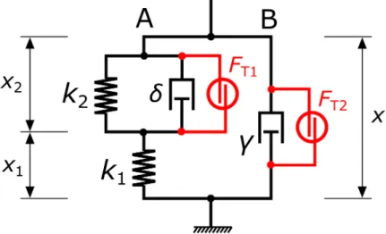
The equivalent mechanical model, which consists of ideal spring and dashpot elements (shown in Figure2), contains two parts. The left branch (A) stands for the nanowire forces exerted on the microbead. The photopolymer viscoelastic properties are characterized by the two elastic termsk₁,k₂and the viscoelastic damping coefficientδ. The right branch (B) includes the damping of the surrounding medium, withγdenoting the hydrodynamic resistance. The inertia of the particle and the displaced fluid are neglected. Therefore, the results obtained represent a low-frequency approximation [20].

Figure 2.The schematic depiction of the linear mechanical model for the microbead motion. Arms A and B represent the nanowire and the hydrodynamic damping by the surrounding medium, respectively. The internal characteristicsx₁,x₂are related to the total observable parameterx.

The basic mechanical model (i.e., model depicted in Figure2, which is free of ran- dom forces FT1 = FT2 = 0) is identical to the one given in [25]. This original form is amended here by adding stochastic forces to the system. In agreement with the fluctuation- dissipation theorem, uncorrelated Gaussian random forces (F_T1andF_T2) are introduced in parallel with the dissipative elementsδandγ. Due to random excitation terms, the two displacement coordinatesx₁andx2fluctuate stochastically, which translates to the overall microbead displacementx = x1+x2. Unlikex1andx2, the value of x can be observed experimentally. The power spectral density and the autocorrelation function of the mi- crobead stochastic oscillations are derived by solving the system of Langevin equations describing the proposed model.

Research Design

Technological advances in microprinting 3D polymer patterns can stimulate and motivate progress in the formulation of appropriate mathematical and physical models.

In this paper, we present a research framework associated with advanced two-photon

microfabrication that can be applied in both practical and theoretical directions. Linear relationships are used to characterize the viscous and elastic properties of micromechanical systems (microbead nanowire systems) operating under stochastic (thermal) dynamic conditions. To evaluate observable coordinate changes, digital data from a CMOS image sensor is processed. This data can be represented mathematically as a one-dimensional time series.

The present study is motivated by experimental results, which, after analyzing the power spectral densities of the corresponding time series, show a kind of double Lorentzian form. The double Lorentzian form of the spectrum appears to us as an attractive research problem but also as a feature that has not yet been explored under the experimental conditions described above.

We use a regression approach with an objective function containing position-dependent weights in the spectrum to compare the theoretical model with experiments and perform the best model parameter finding as well. In addition, our analysis focuses on a validation strategy based on comparisons of differently obtained spectral moments.

Our study reflects the assumption that statistical mechanics models can reveal efficient ways to parameterize optically fabricated systems that exhibit significant fluctuations due to their size.

3. Model

The model consisting of two first-order stochastic differential equations is obtained based on the following considerations: (i) the forces acting in the upper and lower part of branch A are equal, and (ii) the sum of branch A and branch B forces is zero. We study the stochastic system for two displacement coordinates

δdx2

dt +k₂x₂−k₁x₁= F_T1, γ

dx₁ dt +^dx2

dt

+k₁x₁= F_T2

(1)

formulated for the uncorrelated stationary Gaussian and white noise in timetrandom forcesF_T1(t)_,F_T2(t). In such a framework, a set of assumptions applies to the mean values

hFT1(t)i=0 , hFT2(t)i=0 , hF_T1(t)F_T2(t+t⁰)i=0 for all t,t⁰ ; hFT1(t)FT1(t+t⁰)i=CFT1δˆ(t⁰) , hFT2(t)FT2(t+t⁰)i=CFT2δˆ(t⁰)

(2)

written by means of the Dirac delta function ˆδ(.)(Here, the label ˆδis selected to distinguish it from the parameterδ). The details and the physical rationale regarding the new parameter pair CFT1,CFT2will be provided later in Section4.3. To indicate the mean value in the space of repetitive random variants, we use the symbolh. . .i, which is identified with the physical literature. Important here is the mathematical note that random forces are the derivatives of the corresponding Wiener processes.

4. Results

4.1. Solution of the Stochastic Problem

Using a linear transformation involving multiplication by the terms 1/δ, 1/γ, as well as subtraction to remove the combination of derivatives on the left-hand side, we obtained a more standard form of the stochastic differential equation

d dt +k1

1 γ+¹

δ

x1− ^k2

δx2= FS1, d

dt+^k2 δ

x₂− ^k1

δx₁= F_S2,

(3)

where the respective dissipative terms (∼dx1/dt,∼dx2/dt) are counterbalanced by the auxiliary random forcesFS1,FS2. There are no more mixed derivatives of variables in one equation, which results in a qualitative change from white to colored noise. The properties ofF_S1,F_S2can be represented by the linear relations

F_S1(t) = ^FT2(t)

γ −^FT1(t)

δ , F_S2(t) = ^FT1(t)

δ . (4)

For computational purposes, the system of Equation (3) is converted to the Fourier domain in a standard way. Fourier images (coefficients), which we begin to denote by a tilde become functions of the angular frequencyω. Despite the fact that . . ._(ω)or . . .(ω) symbols implying frequency dependence may be redundant in the case of white noise, it emphasizes the dependence onωfor general reasons in other situations. It is also worth noting that the complex conjugate’s asterisk label appears after the transition to the Fourier representation. Assuming that cross-correlations of Fourier images ˜FT1, ˜FT2vanish as a result of Equations (2) and (4), for the relations of the first and the second-order moments, we have

hF^˜_S1i_(ω)=hF^˜_S2i_(ω)=0, hF^˜_S1^∗F˜S1i_(ω)= ¹

γ²hF^˜_T2^∗ F˜T2i_(ω)+ ¹

δ²hF^˜_T1^∗ F˜T1i_(ω), hF^˜_S2^∗F˜S2i_(ω)= ¹

δ²hF^˜_T1^∗ F˜T1i_(ω), hF^˜_S1^∗F˜_S2i_(ω) =hF^˜_S2^∗F˜_S1i_(ω)=− ¹

δ²hF^˜_T1^∗ F˜T1i_(ω).

(5)

Of course, the properties of the above averages are sufficient to determine multivariate Gaussian random force statistics. More precisely, the consequences of the Gaussian process from the postulates forF_T1,2towards the statements forF_S1,2can be easily justified.

According to the Equation (3), the respective coefficients ˜x1(ω), ˜x2(ω), ˜F_S1(ω), ˜F_S2(ω) are present in

G(ω)

x˜₁(ω)

˜ x₂(ω)

=

F˜_S1(ω) F˜_S2(ω)

, (6)

where

G(ω) =

"

iω+k1

1

γ+¹_δ −^k_δ²

−^k_δ¹ iω+^k_δ²

#

. (7)

Note that here G(ω) is the label of newly introduced ω-dependent matrix. The linearity of the problem implies that the solution

x˜1(ω)

˜ x₂(ω)

= G⁻¹(ω)

F˜S1(ω) F˜_S2(ω)

(8)

can be expressed in the terms of the inverse matrixG⁻¹(ω). The following elements of the matrix represent a solution of the linear response type

G⁻¹

11(ω) = ¹

det(G(ω))

iω+^k2

δ

, G⁻¹

12(ω) = ¹

det(G(ω)) k2

δ , G⁻¹

21(ω) = _det(G(ω))^{1 k1}

δ , G⁻¹

22(ω) = _det(G(ω))^{1 h}iω+k₁

1 γ+¹

δ

i .

(9)

We see that the formulas contain det(G) =G_R+iG_I, in the form 1/det(G) = (G_R− iG_I)/(G_R²+G²_I)with the auxiliary real-valued componentsG_R(ω)andG_I(ω). We also state that

G_R(ω) =−ω²+^k1k2

γδ , G_I(ω) =ω k2

δ +k1

1 γ+¹

δ . (10)

Next, we will use

(det(G))^∗ det(G) =G²_R+G²_I (11) often reflected in the results.

4.2. Statistical Averages, Responses to Random Perturbations

This section is about the change to mean values, which are important for the mea- surement process, interpretation, and data processing. Only the statistics of the sum

˜

x1(ω) +x˜2(ω), not isolated ˜x1(ω), ˜x2(ω) is observable in the experiment and allows comparison with the model. Thus, for many aspects of the study, only the behavior of

˜

x₁(ω) +x˜₂(ω)needs to be used to determine experimentally relevant correlations. To understand the statistics ofx, we focus on the Fourier spectrum of autocorrelation function

Cxx(ω)≡ h ( x˜₁^∗(ω) +x˜^∗₂(ω) )( x˜1(ω) +x˜2(ω) ) i

= hx˜^∗₁x˜1i_(ω)+hx˜^∗₂x˜2i_(ω)+hx˜^∗₁x˜2i_(ω)+hx˜₂^∗x˜1i_(ω) . (12) It is of course convenient to divide it into four independent terms. In the following, these are treated independently by means of Equation (8). Partial results (so far without an emphasis on theωdependence) are

hx˜₁^∗x˜1i=(G⁻¹)₁₁^∗ (G⁻¹)₁₁hF^˜_S1^∗F˜S1i+ (G⁻¹)^∗₁₁(G⁻¹)₁₂hF^˜_S1^∗F˜S2i +(G⁻¹)₁₂^∗ (G⁻¹)₁₁hF^˜_S2^∗F˜S1i+ (G⁻¹)^∗₁₂(G⁻¹)₁₂hF^˜_S2^∗F˜S2i, hx˜₂^∗x˜2i=(G⁻¹)₂₁^∗ (G⁻¹)₂₁hF^˜_S1^∗F˜S1i+ (G⁻¹)^∗₂₁(G⁻¹)₂₂hF^˜_S1^∗F˜S2i

+(_G⁻¹)₂₂^∗ (_G⁻¹)₂₁hF^˜_S2^∗F˜_S1i+ (_G⁻¹)^∗₂₂(_G⁻¹)₂₂hF^˜_S2^∗F˜_S2i, hx˜₁^∗x˜₂i=(_G⁻¹)₁₁^∗ (_G⁻¹)₂₁hF^˜_S1^∗F˜_S1i+ (_G⁻¹)^∗₁₁(_G⁻¹)₂₂hF^˜_S1^∗F˜_S2i

+(G⁻¹)₁₂^∗ (G⁻¹)₂₁hF^˜_S2^∗F˜_S1i+ (G⁻¹)^∗₁₂(G⁻¹)₂₂hF^˜_S2^∗F˜_S2i, hx˜₂^∗x˜₁i=(G⁻¹)₂₁^∗ (G⁻¹)₁₁hF^˜_S1^∗F˜_S1i+ (G⁻¹)^∗₂₁(G⁻¹)₁₂hF^˜_S1^∗F˜_S2i

+(G⁻¹)₂₂^∗ (G⁻¹)₁₁hF^˜_S2^∗F˜S1i+ (G⁻¹)^∗₂₂(G⁻¹)₁₂hF^˜_S2^∗F˜S2i.

(13)

We can achieve a clearer relationship by including the correlations between the initially imposed random forces ˜F_T1and ˜F_T2 from Equation (5). The pairwise correlations take the form

hx˜^∗_s x˜mi= hF^˜_T2^∗ F˜T2i

γ² +hF^˜_T1^∗ F˜T1i δ²

!

g_1;s,m+hF^˜_T1^∗ F˜T1i

δ² g_2;s,m (14)

withs∈ {1, 2};m∈ {1, 2}, which define the following eight coefficients g_1;1,1=gˆ_11,11, g_2;1,1=gˆ_12,12−gˆ^sym_11,12,

g_1;2,2=gˆ21,21, g_2;2,2=gˆ22,22−gˆ^sym_21,22,

g_1;1,2=gˆ11,21, g_2;1,2=gˆ12,22−gˆ11,22−gˆ12,21, g_1;2,1=gˆ21,11, g_2;2,1=gˆ22,12−gˆ21,12−gˆ22,11.

(15)

For the relations above, we use a notation that also includes the auxiliary symbols ˆg_ij,kl and ˆg_ij,kl^sym. They are interrelated to the combinations(G⁻¹)^∗_ij(G⁻¹)_ijof the priorG⁻¹terms gˆij,kl= (G⁻¹)^∗_ij(G⁻¹)_kl , gˆ_ij,kl^sym=gˆij,kl+gˆkl,ij . (16) Obviously, the emphasis on the symmetry ˆg_ij,kl^sym= gˆ_kl,ij^sym will help us to handle the complex numbers. Furthermore, we recognize that the identical pairs of indices provide that ˆgij,ij= (1/2)gˆ^sym_ij,ij. The advantage of the auxiliary notation by means of ˆg...is that we obtainCxxfrom Equation (12) in the compact form

Cxx = hF^˜_T2^∗ F˜T2i γ²

ˆ

g11,11+gˆ21,21+gˆ_11,21^sym + hF^˜_T1^∗ F˜_T1i

δ² ( gˆ_11,11+gˆ_12,12+gˆ_21,21+gˆ22,22 (17) + gˆ_11,21^sym +gˆ_12,22^sym −gˆ_11,12^sym −gˆ_21,22^sym −gˆ_11,22^sym −gˆ_12,21^sym

. We continue the calculation to reveal the terms introduced by Equation (16)

ˆ

g11,11= _G2¹

R+G²_I

ω²+^k_δ²²

, gˆ21,21= _G2¹

R+G_I²

_k

1

δ

2

, gˆ22,22= ¹

G²_R+G²_I

ω²+_k²₁¹

γ+¹

δ

2

, gˆ12,12= ¹

G_R²+G_I²

_k

2

δ

2

,

(18)

ˆ

g_11,21^sym = _G2¹

R+G_I²

_2k

1k₂ δ²

, gˆ_12,22^sym = _G2¹

R+G²_I

_2k

2k₁ δ

1 γ+¹_δ, ˆ

g_11,12^sym = _G2¹

R+G_I²

2k²₂ δ²

, gˆ_21,22^sym = _G2¹

R+G²_I

2k²₁ δ

1 γ+¹_δ, ˆ

g_11,22^sym = _G2¹

R+G_I²

h2ω²+^2k1k2

δ

1 γ+¹

δ

i, gˆ_12,21^sym = _G2¹

R+G²_I

_2k

1k₂ δ²

.

(19)

Note that we usedG_RandG_Ifrom Equation (10) to express the result. After substitut- ing these elements into Equation (17), we come to the relation

Cxx(ω) = ¹ γ²(G²_R+G²_I)

(

hF^˜_T2^∗ F˜T2i

"

ω²+

k1+k2

δ 2#

+hF^˜_T1^∗ F˜T1i k1

δ 2 )

, (20) which is important to derive measurable results. We will apply a similar procedure later to determine the pairwise correlations to prove the validity of the equipartition theorem.

4.3. Towards Fusing of Theory and Experiment

Suppose that there are two finite formal limits relevant for the obtaining of the power spectral density in the form

CFT1= lim

Tmsr→∞

hF^˜_T1^∗ F˜T1i

Tmsr , CFT2= lim

Tmsr→∞

hF^˜_T2^∗ F˜T2i

Tmsr . (21)

The formula is understood as a postulate, which introduces the duration of the measurement timeTmsr[19] into a part of the procedure at the formal level. The correlations in the Fourier domain can be formally taken as infinite for frequencyf = _2π^ω 1/Tmsr. The formal nature of the limits given by Equation (21) makes it evident that considerations are not fully compatible with the Fourier framework because the measurement is dependent on assumptions about the large time (Tmsr) of the measurement.

The occurrence of C_FT1 and C_FT2 later in Equation (23) can be interpreted as the contribution of the power spectral densities of two random force variants given by the Wiener–Khinchintheorem

T_msrlim→∞

hF^˜_Tj^∗F˜_Tji Tmsr

= Z _∞

−∞dt⁰e^{−2πi f t0}hF_Tj(t)F_Tj(t+t⁰)i=C_FTj (22) considered forj = 1, 2 alternatives (see Equation (2), where the correlation function is defined and integrated). If we extend the application of the formal limit by dividing Equation (20) withTmsr, we obtain the power spectrum density in the form

Sxx(f) = lim

T_msr→∞

Cxx(f) Tmsr

= ¹

γ²(G²_R+G²_I)_ω=2πf (

CFT2

"

4π²f²+

k1+k2

δ

2# +CFT1

k1

δ 2)

. (23)

In this way, the physical meaning of the coefficientsCFT 1,2is revealed. They can also be represented in an independent way by expressing their relation to the absolute temperature CFT1=2kBTδ, CFT2=2kBTγ. (24) However, this construct also provides information about the dissipative mechanisms.

This is built with the idea that fluctuations from random forces are dissipated by the mechanisms represented by the parametersδ,γ. As provided below in Section4.5, the mean potential energy for the respective degrees of freedom can be compared to determine the equilibrium level of energy flow controlled byCFT1andCFT2. The Equation (24) given above is essentially the case of the generalfluctuation–dissipation theoremintroducing the natural heat unitk_BT.

The fluctuation–dissipation theorem is a statistical thermodynamics statement that explains how fluctuations in a detailed balanced system determine its response to applied disturbances. According to this theorem, two opposing mechanisms are responsible for creating a detailed equilibrium in mechanical systems. On the one hand, there are the consequences of the dynamics of a microsphere attached to a nanowire that is damped by the surrounding fluid. Contributions from the internal damping mechanisms of the nanowire also fall into the same category. Even with this damping combination, the me- chanical energy is converted into heat. On the other hand, the presence of damping is necessarily accompanied by fluctuations born in the viscous environment. In the case of the surrounding liquid, these fluctuations result in typical random Brownian collisions of liquid molecules with the microbead. In a standard way, the process is interpreted so that on microscopic scales, heat can be converted back into the mechanical energy of the microbead. The internal damping inside the nanowire acts likewise. Summarizing the above statements, we arrive at a specific form of the fluctuation-dissipation theorem, which

states that a constant dissipation flux keeps the mean mechanical energy input invariant, while ensuring the production of new fluctuations.

As a result, let us emphasize an important point: Equation (23) can be modified to account for the temperature effect. With the intention of linking theory with experiment, we attain the expression

Sxx(f) = ^2kBT γ

4π²f²+K_A

(4π²f²−K_B)²+4π²f²K_C. (25) The asymptotic, high-frequency consequence of this general result is

Sxx(f)' ^kBT

2π²γf², f ¹ 2πmax

(

pKA,p KB,p

KC

)

. (26)

At this stage, we benefit from the choice of auxiliary parametersKA,KB,KC. Returning to material details is possible using transformations

KA=

k1+k2

δ 2

+^γ δ

k1

γ 2

, KB= ^k1k2

γδ , KC= k2

δ +k1

1 γ+¹

δ 2

. (27) These auxiliary parameters are positive for a given model specification that operates exclusively with positivek1,k2,δ,γ. However, there is also another, more sophisticated level of interpretation. It is interesting and also productive to assume that the result can be written as a sum of two weighted Lorentzian functions

4π²f²+KA

(4π²f²−KB)²+4π²f²K_C

=! ¹

Γ2−Γ1

KA−_Γ1

Γ1+4π²f² + ^Γ2−KA

Γ2+4π²f²

. (28) HereΓ1,2 play the role of free parameters, which incorporate information coming from previously introduced KA, KB, KC. The change toΓ1,2 should be considered as an intermediate step along with other consequences. The key consequence is double Lorentzian form

Sxx(f) = ^kBT 2π²γ(f_C2² −f_C1² )

K_A 4π² −f_C1²

f_C1² +f² + ^f

2 C2−_4π^KA₂ f_C2² +f²

!

. (29)

It is based on the assumption that there exist some relations betweenΓ1,2and the corner frequenciesf_C1,2. When Equations (28) and (29) are combined, we obtained

f_C1,2² = ^Γ1,2 4π² = ¹

4π² K_C

2 −K_B∓¹ 2

q

K_C(K_C−4K_B)

. (30)

In the above solution, we use the consensus that the plus sign corresponds to fC2. The constraints that allow for such a solution are as follows:

KC

2 −KB≥ ¹ 2

q

KC(KC−4KB), KC≥0 , KC≥4KB. (31) If we consider the transformation to physical parameters in the sense of Equation (27) to analyze the satisfaction of the above constraints, we obtain

K_C

2 −K_B = ^k

21

2 1

γ+¹ δ

2

+^k1k2 δ² + ^k

22

2δ² ≥0 , (32)

K_C−4K_B = k₂

δ − ^k1 γ

2

+ k₁

δ 2

+^2k1 δ

k₂ δ +^k1

γ

≥0 . (33)

Using Equation (27), we confirm thatK_C≥0. Moreover, the trivialK²_B≥0 implies (K_C/2)−KB≥(1/2)^pK_C(K_C−4KB). Therefore, there is no obvious contradiction with the fact thatΓ1,Γ2correspond tof_C1² ,f_C2² . It is also notable that the inverse transformations (fC1,fC2)→(Γ1,Γ2)→(KB,KC)become

KB=^pΓ1Γ2=4π²fC1fC2 , K_C=2

pΓ1Γ2+^Γ1+Γ2

2

=4π²(f_C1+f_C2)². (34) The result is intriguing in terms of revealing the central tendency inKB(_Γ1,Γ2)and KC(Γ1,Γ2)as representatives of the pairΓ1,Γ2.

4.4. Autocorrelation Function

The findings presented above can be augmented by using direct time representation.

According to the well-knownWiener–Khinchinrelation, we have the consequence for the autocorrelation function in the form

Rxx(t) = Z _∞

−∞df Sxx(f)exp(2πi f t). (35) As a result, for Equation (29) as a specific version ofSxx(f), we obtain a two-exponential autocorrelation function

Rxx(t) =R₀R₁e^−2πfC1|t|+R₂e^−2πfC2|t|

, (36)

where

R₀= ^kBT

2πγ(f_C2² −f_C1² )^, R₁=

K_A 4π² − f_C1²

fC1 , R₂= ^f

2 C2−_4π^KA₂

fC2 . (37)

It is worth noting that corner frequency parameters have a significant impact on autocorrelation decrease over time. At a first glance, we can see the essential property here where a pair of frequencies in the Lorentz form corresponds to a pair of damping terms with the typical decay times proportional to 1/fC1and 1/fC2. It should also be noted that, assuming that the physical parameters are constant, the temperature is directly manifested only in the amplitudeR₀. The calculations above were performed with the help of a well-known auxiliary relation

Z _∞

−∞df exp(2πi f t) f²+f_C² = ^π

f_Cexp(−2π|t|f_C) (38) with some auxiliary parameter f_C.

4.5. Sharing of Elastic Energy; Rationale for Choosing CFT1, CFT2

According to the principle of energy equipartition, average energy is evenly dis- tributed among the various degrees of freedom of ergodic systems. As shown here, the im- plications of this principle are valuable tools for calculating the amplitudes(CFT1,CFT2) of a pair of random forces. The equipartition principle can be applied to the mean elastic energies. We start by writing the energy for the Fourier modes corresponding toω. It is worth noting that since the inertial term is considered negligible, the zero limit of the kinetic energy has no effect on the equipartition issues.

Using the integration techniques already discussed, we continue to utilize the formal limit approach (Tmrs → ∞) for the integration of the spectrum and averaging over the respective potential energy fluctuations as follows

U_P1= ^k1 2

Z _∞

0 dω hx˜₁^∗x˜₁i_(ω)= I_P11C_FT1+I_P12C_FT2, U_P2= ^k2

2 Z _∞

0 dωhx˜^∗₂x˜₂i_(ω)=I_P21C_FT1+I_P22C_FT2 .

(39)

The formulas below can be applied to complete the integration I_P11 = ^k1

2δ²I_E2, I_P12 = ^k1

2γ²

I_E2+^k2

δ

2

I_E0

, I_P21 = _2δ^k2₂

I_E2+^k1

γ

2

I_E0

, I_P22 = _2γ^k2₂^k21

δ²I_E0 .

(40)

These four coefficients include two spectral integrals I_E0=

Z _∞ 0

dω π

1

G²_R(ω) +G_I²(ω)^{, IE2}= Z _∞

0

dω π

ω²

G²_R(ω) +G_I²(ω)^{. (41)} Going back to a spectral decomposition using a pair of Lorentzian forms (see Equation (29)) in combination with Equations (30) and (34) gives the following result

I_E0= ¹ 2(Γ2−Γ1)

1

√Γ1

−√¹ Γ2

= ¹

2KB

√KC

, IE2= ¹

2(Γ2−Γ1)

pΓ2−^pΓ1

= √¹ KC

.

(42)

As a consequence, the following relationshipIE2=IE0k1k2/(γδ)can be used in the mean potential energies listed below

UP1= ^k1k2 2γδ

k1

δ CFT1

δ + k1

γ +^k2 δ

CFT2

γ

IE0, UP2= ^k1k2

2γδ k1

γ + ^k2 δ

CFT1

δ + k1

δ CFT2

γ

IE0 .

(43)

Finally, in accordance with Equation (24), we have the confirmation of the equipartition in the form

UP1=UP2=KB

pK_CIE0kBT= ¹

2kBT . (44)

4.6. The Spectrum Moments

In this subsection, we discuss the usefulness of introducing power spectral density integrals in cases where the frequency domain over which we integrate is divided into non-intersecting intervals. Frequency integration is motivated by the fact that providing excessive detail for spectrum characterization may be unnecessary in certain contexts. The second reason is that aggregation of data helps to suppress statistical errors. The third reason is the possibility of comparing only a few moments with the moments estimated by direct data processing.

Naturally, the analytical form of the model moments simplifies further processing.

In our case, the specificity of the moments corresponding to Lorentzian and related spectral forms supports the overall validation process. Let the regression-related (rr) moments obtained by analytical integration be referred to asM^rr_Sxx(f_L,f_H). This notation is used to

mean that integration has occurred within the range between the lowest f_Land the highest f_Hfrequencies. Then

M^rr_Sxx(f_L,f_H) = Z f_H

f_L df Sxx(f)

= R₀ π

R₁

arctan

fH

f_C1

−arctan fL

f_C1

(45) +R₂

arctan

fH

f_C2

−arctan fL

f_C2

.

Because the interval length may diverge, we decided to use non-normalized moments.

Recall thatR₁andR₂are the two respective amplitudes of the exponentials corresponding to the autocorrelation function (see Equation (37)). On this basis, using fC1, fC2as natural boundaries, we can define the system of three specificregression-relatedspectral moments M^rr_Sxx(0,fC1) = R₀

π

R₁^π

4 +R₂arctan fC1

f_C2

, M^rr_Sxx(fC1,fC2) =R₀

π

R₁arctan fC2

f_C1

− R₂arctan fC1

f_C2

+ (R₂− R₁)^π 4

, (46)

M^rr_Sxx(fC2,∞) = R₀ π

(2R₁+R₂)^π

4 − R₁arctan fC2

f_C1

with the total sum(1/2)R₀(R₁+R₂). Other suitable boundary options are, of course, possible, such as those that do not depend on regression results but instead emerge entirely from generalized averaging procedures of the experimental spectrum.

4.7. Experimental Results and Their Regression

After the successful implementation of the experiment, we obtained data representing the observed dynamicsx(t), which we have then transformed into corresponding Fourier images. The aim was to obtain an experimental power spectrum density{S^ex_xx,j}^N_j=1^ex for the system ofN^exfrequencies{fj}^N_j=1^ex(see Figure3). Some of the evaluations have been performed according to the work of [19]. Preprocessing with grouping of the adjacent experimental spectral points is a necessary methodological peculiarity. Frequency and spectrum groupings with eight points over the frequency decade were introduced. The effectiveness with which the representative grouping frequencies were allocated was eval- uated. Naturally, the grouping process affects not only the locations of representative frequencies, but also the statistics of spectral points, potentially increasing the regression’s feasibility. The optimization of parametric combinations is made possible by data knowl- edge. Let us formally encapsulate the unknown model parameters in a single symbol Par, resulting in the parameterized form of the double Lorentzian modelSxx(f_j,Par)(see Equation (29)). In addition to identifying the optimum, we will focus on estimating errors for various components ofPar.

The problem-specific emphasis is on the asymptotic behavior of the spectrum. Despite the fact that the density of the power spectrum decreases as∼ f⁻², the high frequency domain must be properly included in the regression due to its physical significance. Hence, a weighted regression of the squares ofSxx(f_j,Par)−S^ex_xx,jdeviations has been implemented.

The preference can be defined as the minimization of the objective function

Obj_F(Par)≡

N^ex j=1

∑

"

Sxx(f_j,Par)−S^ex_xx,j S^ex_xx,j

#2

. (47)

Here, the parameters and their combinations appear to be formally merged into the vector

Par≡

fC1, fC2, KA

4π², kBT 2π²γ

. (48)

This is subject to optimization. We used the standard global function optimizer, which was built on the concept of the [26] work with the implementation (scypy.optimize.curve- _fit(. . . )) to the SciPy library [27]. The regression corresponding toObj_Fprovides the corner frequencies

fC1= (0.443±0.093) (Hz), fC2= (4.82±0.23) (Hz). (49) Along with them

K_A

4π² = (0.47±0.19) (Hz²). (50) Finally, there is also fixed corresponding parametric combination

kBT

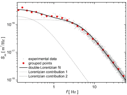
2π²γ = (3.53±0.13)×10⁻¹⁵(m²Hz), (51) which represents the constant factor inSxx(f,Par)as defined by Equation (29). The regres- sion outcomes are depicted in Figure3.

Figure 3.Power spectral density of microsphere fluctuations. The solid line belongs to the model according to Equation (29). The fit was set after optimization ofObj_F(Par). Two Lorentzian contributions spanning the entire spectrum are also shown.

Now there is a standard way to find out the autocorrelation function (see Equation (37)) via the respective parameters

R₀ π =

_k

BT 2π²γ

f_C2² − f_C1² =_1.532×10⁻¹⁶ (_m²_/Hz)_, R₁=_0.623(_Hz)_, R₂=_4.723(_Hz)_.

(52)

A posteriori evaluation methodology following the regression results provides an implication for the values of theregression-relatedspectral moments

M^rr_Sxx(0,fC1) = 1.414×10⁻¹⁶(m²),

M^rr_Sxx(f_C1,f_C2) = 5.682×10⁻¹⁶(m²), (53) M^rr_Sxx(f_C2,∞) = 5.772×10⁻¹⁶(m²).

We see that the sum of the moments 1.286×10⁻¹⁵ (m²)equals(R₀/2) (R₁+R₂), as predicted.

Adjusting the integration boundaries can be important for the design of some al- ternative test moments. The premise of the adjustment is that these variants should be more closely linked to the measurement process, conditioned by the need to avoid spectral distortions known as “aliasing” and “motion blur”. The effects occur due to too superficial and insufficient sampling of the signalx(t)captured by the camera. This means that the calculations must focus on bands with frequencies less than fupp, which in our case was set to around a quarter of the Nyquist frequency. The lower limit value flowprevents the use of extremely low frequencies. Respecting the lower limit suppresses distortions caused by the apparatus background noise. Numerically, the boundaries we introduce are

f_low=0.1333[Hz]and fupp=59.97[Hz]. The following three moments M^ex_Sxx(f_low,fC1) = 0.924×10⁻¹⁶(m²),

M^ex_Sxx(f_C1,f_C2) = 5.687×10⁻¹⁶(m²), (54) M^ex_Sxx(f_C2,fupp) = 4.952×10⁻¹⁶(m²)

were created to express the properties of the experimental data set, which was achieved by partly reducing the impact of the regression results. Here we see that Simpson’s integration quadrature based on uniform data sampling (without grouping) also provides us with variants of spectral moments. However, even when using numerical integration, we must be careful if we subsequently perform comparisons and interpretations. The reason is that certain integrals approximated by a suitable summation can become dependent on the previous regression only by their integration boundaries when these are linked to regression parameters (fC1and fC2). Independence from regression can be achieved using descriptive spectrum characteristics (analogous to descriptive statistics). This means using characteristic frequencies in the role of integration boundaries. Then the results of the calculation are generalized spectral averages. The fact that we do not present more moment variants here is mainly related to the focus of this work.

When comparing the Equations (53) and (54), we see that only the central moments for the[fC1, fC2]band are close enough to each other, which means thatM^rr_Sxx(0,fC1)and M^rr_Sxx(f_C2,∞)are not sufficient approximations ofM^ex_Sxx(f_low,f_C1)_andM^ex_Sxx(f_C2,fupp)_, respectively. Results show that in the case of regression-related moments, there is only a slight and negligible rise in moments compared to the use of Simpson’s rule

∼ 1.2 % increase : (55)

M^rr_Sxx(0,f_C1)− M^rr_Sxx(0,f_low) = 0.935×10⁻¹⁶(m²)

& M^ex_Sxx(f_low,f_C1),

∼ 4.6 % increase :

M^rr_Sxx(f_C2,∞)− M^rr_Sxx(fupp,∞) = 5.184×10⁻¹⁶(m²)

& M^ex_Sxx(fC2,fupp).

5. Discussion

Two kinds of spectral moments (M^rr_Sxx(.)andM^ex_SSx(.))were designed, calculated and compared for the experimental input data given. We have shown by analysis that