Discrete Applied Mathematics

(1)

Contents lists available atScienceDirect

Discrete Applied Mathematics

journal homepage:www.elsevier.com/locate/dam

Arrival time dependent routing policies in public transport

Kristóf Bérczi

^a,b,

* , Alpár Jüttner

^a,b

, Marco Laumanns

^c

, Jácint Szabó

^c

aMTA-ELTE Egerváry Research Group, Budapest, Hungary

bDepartment of Operations Research, Eötvös Loránd University, Budapest, Hungary

cIBM Research, Rüschlikon, Switzerland

a r t i c l e i n f o

Article history:

Received 30 November 2016 Received in revised form 8 May 2018 Accepted 11 May 2018

Available online xxxx

Keywords:

Public transport Routing policy

Stochastic route planning Utility function

a b s t r a c t

We present a routing system that considers uncertainties, which are prevalent in any real transport system. Given desired departure or arrival times and a utility function representing the traveller’s preferences, our method computes not just a single path through the network, but a more sophisticated and adaptive journey plan called routing policy. For each stop and time instance, a policy specifies the list of services that the passenger is recommended to take.

We show that the problem of finding an optimal policy is NP-hard. We also give a polynomial-time algorithm for a relaxation of the problem when the number of recommended services is limited at each stop and time. A computational case study for the public transport network of Budapest shows that the obtained routing policies can lead to substantial travel time savings compared to deterministic plans, and that considering multiple service policies leads to an improvement compared to previous solutions using single-service policies.

1. Introduction

Public transport plays an essential role in reducing the traffic load, but disturbances due to congestion as well as planned or unplanned events such as maintenance work or accidents can have strong effects on travel times of public transport vehicles and its quality of service. As a result, public transport is often perceived as unreliable and therefore not always used to its full potential.

Journey planning is a key process in public transport, where travellers get informed how to make the best use of a given system for their individual travel needs. Nowadays, public transport providers routinely offer journey planning applications either on their websites or via mobile applications. For a given journey request, these applications usually offer one or several routes, which are linear sequences of activities or legs that form the itinerary. A common trait of the underlying journey planning algorithms is that they assume a deterministic environment. However, as changing traffic conditions can have strong effects on travel times, vehicles in public transport often deviate from their schedule.

On the other hand, there are often multiple alternative services which a passenger can choose from at a given location.

Public transport providers have started to take advantage of such options and offer dynamic journey planning capabilities, for example push services to alert travellers of broken connections and to deliver updated journey plans by re-planning the journey anew from the current location and based on the current traffic conditions. Despite providing some adaptability, linear journey plans are not able to capture the full amount of flexibility inherent in multi-service public transport systems, because re-planning always occurs after some deviation from the assumed original conditions has occurred.

*

Corresponding author at: MTA-ELTE Egerváry Research Group, Budapest, Hungary.

E-mail addresses:berkri@cs.elte.hu(K. Bérczi),alpar@cs.elte.hu(A. Jüttner),mlm@zurich.ibm.com(M. Laumanns),mlm@zurich.ibm.com(J. Szabó).

(2)

To fully exploit the given flexibility and to pre-plan adaptive decisions accordingly, we propose to use the concept of a routing policy instead of a linear journey plan. A routing policy is a state dependent routing advice at each location. A routing advice may consist of more than one service and specifies exactly which service to take in each situation. The traveller may define an arrival time dependent utility value at the destination, representing her preferences regarding arrival time deviations and delays. The goal is to find a policy that maximizes the expected value of the utility that can be achieved by following the policy.

Previous work.Finding shortest paths in a network with respect to given arc travel times is a central problem in combinatorial optimization. The fundamental results of Dijkstra [9], Bellman [3], Ford [14] and Floyd [13] are well-known examples of route planning algorithms. Due to their wide applicability, improved versions of these algorithms were introduced, e.g. the A* algorithm by Hart et al. [19], which is the basis of many street map based route planners. A common property of these algorithms is that they work with static arc travel times and provide a single route as a solution.

There have been various attempts to address uncertainty in routing problems. The travel time of an arc can be modelled as a random variable with a given probability distribution. In this model the effectiveness of a route can be measured in many ways: both the expected travel time and the reliability are worth to be considered. When time-independent distributions are assumed, one can take the mean travel times and find the path with minimum expected travel time by Dijkstra’s algorithm.

Time-dependent distributions have also been considered. In [18], Hall showed that standard shortest path algorithms do not necessarily find minimum travel time paths in this case. He introduced a ‘time-adaptive decision rule’ in which the next node is defined for each step as a function of the arrival time to the node. However, mostly heuristics are known for these problems, see for example [2,27].

A more general framework is obtained if the quality of a route is measured in terms of a utility function. Loui [21] showed that optimal solutions can be found for numerous special cases such as linear, exponential or quadratic utilities. In one of the earliest works, Frank [15] defined a reliable optimal path as a path maximizing the probability of arriving before a given time. This problem was later given the name Stochastic On-Time Arrival (SOTA) problem [10]. Murthy and Sarkar [22] gave an exact solution to the SOTA problem in case the travel times follow normal distributions.

Besides looking for optimal paths, a lot of research has been done for finding optimal routing plans, mainly based on models and techniques from stochastic dynamic programming. A recourse model for stochastic shortest paths was considered in [24]. Fan et al. [10] applied stochastic dynamic programming to find on-line travel plans, where the next arc is computed depending on the travel times on the path already visited. Fan and Nie [12] reformulated the SOTA problem of [15] in terms of stochastic dynamic programming. Their standard successive approximation algorithm converges in acyclic networks, but its running time is unbounded in the general case. In [11] they proposed a pseudo-polynomial discrete approximation algorithm for the same problem, which converges in a finite numbers of steps. Hoy and Nikolova [20]

presented a dynamic programming algorithm to find approximately optimal arrival time dependent paths in directed acyclic networks. Results on the SOTA problem were theoretically and numerically further improved by Samaranayake et al. [25].

The computational difficulties come from the fact that continuous-time convolution products have to be computed several times, which is hard to solve analytically. Although discretizing the problem might help, the computational effort of the convolution steps remains large; therefore methods speeding up this process are of interest, see e.g. [26].

There is a fundamental difference between individual transport and public transport routing problems. In the individual transport case, due to the absence of transfers, the delay uncertainties on road segments simply add up. Hence, if a distribution is assumed on the arcs that fulfils certain properties, the travel time distribution of a given path can easily be computed. These results cannot be directly applied to the public transport case, where transfers are fundamental elements of the system. Botea et al. [6] and Dibbelt et al. [8] investigated public transport journey planning in the presence of uncertainty.

They proposed a model in which uncertainty appears as estimated times of arrival of transport vehicles and the duration of actions such as walking. In [6] a heuristic solution is found by using Weighted AO* as a baseline search method, extended with different speed-up enhancements. The solution is a probabilistic plan where branches correspond to single choices at a given stop and have probabilities. The quality of the solution is measured in terms of robustness to uncertainty. In [8] a dynamic programming algorithm is given to find an arrival time dependent single choice routing plan minimizing expected arrival time.

If there are multiple services serving the same stop, there might be several good service choices depending on the actual arrival times. Thus, even if we were able to find a single choice with largest expected utility, the solution may be suboptimal.

The difficulty of the problem therefore lies in selecting a set of ‘alternatives’ for each node instead of a single path. This framework was previously studied by Nonner [23] who proposed a method that computes a list of services for each stop depending on the waiting time distributions, and the user is recommended to take the service from the list that arrives first.

As a respective model, Nonner suggested to determine the waiting time distributions as a function of the passing frequencies of the services at a given node. The method is also able to use online data provided by monitoring devices, in order to re- plan and update the lists of alternatives for each stop whenever new information concerning delays, position of a vehicle, unexpected events, or level of congestion arrives. The notion of ‘routing alternatives’ of [23] was further developed by the first author et al. [4]. They adopted the notion of ‘policies’ and provided current time dependent policies consisting of not only a single service but a set of services, so that the resulting travelling advice gets more robust to uncertainty.

Contribution.The aim of the present paper is to examine arrival time dependent policies with multiple service choices for monotone non-increasing utility functions. We formalize the problem and introduce the notion of arrival time dependent policies in Section2. In Section3we show that there always exists an optimal policy, although finding one is NP-hard.

However, if the number of services that a policy may contain is bounded by a constantkfor each stop and time then an

(3)

optimal policy can be found in polynomial-time; the algorithm is discussed in Section4. Section5gives an evaluation of arrival time dependent policies by comparing them to deterministic routing plans through extensive simulations.

2. Stochastic model

In the forthcoming discussion, we use a simplification of real public transport systems. For ease of representation, we assume that the transport system consists of individual services between two nodes, that is, each service has only two stops:

its origin and its destination node. We also assume that the probability of two services arriving to the same stop at the same time is negligible. Of course this simplified set-up gives a very rough model of real public transport systems, but enables the usage of a much simpler, clearer notation and descriptions of the algorithms. It is important to note that the presented methods and formulas can be adapted to the case when services have several stops and the services may arrive to the same stop simultaneously. Accordingly, the computational case study of Section5uses a more complex and realistic model which considers services with several stops, and services are allowed to arrive to a given stop at the same time.

The stochastic model for the public transport network that we consider is the following. Theset of stopsis represented by a set of nodesV. We denote theset of servicesbyS. The set of services leaving from nodevis denoted byS_vand the maximum number of services leaving from any node is denoted by∆= max_v∈_V{|S_v|}. Theoriginanddestination nodesof services∈Sare denoted byosandds, respectively. Thetransport networkis then represented by a directed graphD=(V,^A) wherevw∈Aif and only if there is a services∈Switho_s=v^and^ds=w. The indicator variable of some logical statement is denoted byχ, for example,χ^(x∈X) is 1 ifx∈Xand 0 otherwise.

We consider two kinds of probabilistic data: the probability distribution of arrival and departure times, and the probability distribution of travel times. To characterize these, we introduce the following random variables: given a services, the random variable of the departure time ofsfromo_sis denoted byD_s, the random variable of the arrival time ofstod_sis denoted byA_s, and the random variable of the travel time ofsfromo_stod_sis denoted byT_s. It is assumed that there exists a global constant τ >0 such thatT_s≥τ^{for each}^s∈S. Clearly, we have

A_s=D_s+T_s.

For a given random variableX, we will denote the correspondingcumulative distribution function (CDF)byF_X(t) and the probability density function (PDF), if exists, byf_X(t). Theexpected valueofXis denoted by E[X], while theconditional expected valueofXgiven an eventHis denoted by E[X|H]. IfXis a discrete random variable thenP[X∈Z]denotes the probability of Xhaving a value fromZ.

Our goal is to give advice how passengers should best use the given stochastic transport network for their travel request from a given origin to a given destination. We formalize such a travel advice as a routing policy. Informally, a routing policy assigns a set of services to each stop and time. The set of recommended services depends on the passenger’s arrival time to the stop, and will not change during the stay at the given stop. More precisely, apolicyis a functionP :V×_R→2^Ssuch thatP_v(t):=P(v,^t)⊆S_v. LetV^′ ⊆Vand assume that for eachv ∈V^′a timet_v ∈_Ris given. IfP_v(t) is only defined for t ≥t_vwheret_v∈_Rfor allv∈V, then it is called apartial policy.

The interpretation of a policy is the following. If a passenger arrives to stopv^{at time}^t0and a services∈P_v(t₀) departs at timet > ^t0from stopv, then the passenger is recommended to take the service at timet. Ties among services leaving simultaneously is broken uniformly at random. The set of possible policies is denoted byP.

We will characterize the quality of a policy by the utility it provides to the passenger. Autility functionis a function u:_R→_Rwhich represents the user’s preference according to the time of arrival to the destination node. We assume the existence of a certain ‘deadline’ (t_end) after which the user’s utility is−∞.

Assume that a destination nodevd, a utility functionu:_R→_Rand a policyPare given. For any stopv ∈Vand time t ∈_R, theutility induced byPat stopv^{and time t}is denoted byU_v^P(t). That is,U_v^P(t) denotes our expected utility supposing we arrive to stopv^{at time}^tand we continue our journey according to the policyP. Theconditional utility induced byPand service s at stopv^{and time t}is denoted byU_v^P(t |s) and is defined as our expected utility if we take servicesat stopv^and timet. When considering continuous time, the induced utility can be computed as

U_v^P(t)=

∫ ∞ t

∑

s∈Pv(t)

⎛

⎜

⎝

U_v^P(t^′|s)f_D_s(t^′) ∏

s′ ∈Pv^(t) s′ ̸=s

( 1−

∫ t′ t

f_D_s′(t^′′)dt^′′

)

⎞

⎟

⎠ dt^′,

where

U_v^P(t|s)=

∫ ∞ τ

U_d^P

s(t+t^′)f_T_s(t^′) dt^′.

To circumvent the computational difficulties involved when handling continuous functions, we restrict the problem to a finite time horizonand discretize the planning horizon into small intervals of a few seconds. We can therefore assume that every event happens at timet ∈ [T] = {0,¹, . . . ,^T}, whereT corresponds to the deadline. Consequently, all distributions are discrete on the set{0,¹, . . . ,^T}. In the discrete version, a policy is a functionP : V× [T] → 2^S. The travel time of a service is strictly positive and, as the time is discretized, at least as large as one time interval.

(4)

As we assumed that services do not arrive simultaneously, in the discrete case we have

U_v^P(t)=

T

∑

t′=_t

∑

s∈Pv(t)

⎛

⎜

⎝

U_v^P(t^′|s)P[D_s=t^′] ∏

s′ ∈Pv^(t) s′ ̸=s

⎛

⎝1−

t′−₁

∑

t′′=_t

P[D_s^′ =t^′′]

⎞

⎠

⎞

⎟

⎠ ,

and

U_v^P(t|r)=

T−_t

∑

t′=₁

U_d^P_r(t+t^′)P[T_r =t^′].

Before discussing how to find policies with high expected utility, let us call attention to a peculiar feature of arrival time dependent travel plans. By definition, such a policy solely depends on the arrival time to a given stop and so does not condition on the time until the deadline. However, there might be situations when it is worth reconsidering and changing the set of suggested services according to the amount of time spent at the given stop. Such routing policies, calledcurrent time dependent policies, are also of interest and are considered in [5]. A significant difference between the two approaches is thatoptimalitycan be defined for arrival time dependent policies (see Section3), while an analogue concept does not work for the current time dependent case as an optimal policy may not exist at all. The results of the present paper, including the existence of an optimal policy, are meant when the space of policies is restricted to the arrival time dependent ones.

3. Optimal policies

A policy is calledoptimalifU_v^P(t) ≥ U_v^P^′(t) for eachP^′ ∈ P,v ∈ Vandt ∈ [T]. The notion of an optimal policy is demonstrated by the following example.

Example 1. Assume that the network consists of two nodesv^andwand three servicess₁,^s2ands₃going formv^tow^. The services depart fromvas follows:s₁departs in intervalsI₁andI₂with probability¹₂and induces utility 3,s₂departs in intervalI₃with probability 1 and induces utility 2, ands₃departs in intervalsI₂andI₃with probability¹₂and induces utility 1. Not arriving to stopwat all has utility 0.

In this very simple case it is possible to guess the optimal policy. Note that it makes sense to include a service in the set of recommended ones for a given interval even if the service in question departs with probability 0 as a policy do not change after the passenger’s arrival to the stop.

InI3, the optimal policy consists of the single services2as it arrives with probability 1 and is clearly better thans3. For intervalI₂, the optimal policy containss₁ands₂. Indeed, taking onlys₁would not be enough as it may have already left inI₁. Finally, forI₁the optimal policy consists of the single services₁as it arrives inI₁orI₂with probability 1 and has the highest induced utility.

By definition, the set of recommended services depends only on the arrival time to a given stop. That is, the induced utility does not depend on the policy at the same stop in later time instances. This suggests that an optimal policy may always exist. Beside showing that this impression is indeed true, the proof of the next theorem also provides a recurrence relation between the optimal policies at different times.

Theorem 2.There always exists an optimal policy.

Proof. Recall that the length of a time interval is a strictly positive lower bound for the travel times. Lett ∈ [T]and assume thatPis a partial policy which is already defined for allt^′ >^toptimally, that is,U_v^P(t^′)≥U_v^P^′(t^′) for eachP^′ ∈P,v∈V andt^′>t. Take an arbitrary stopv∈Vand a subsetX⊆S_vof services atv. We define a new partial policyP^Xas follows:

P_w^X(t^′)=

{P_w(t^′) ift^′>^t,

X ift^′=tandw=v.

LetP_v(t)=P_v^X^opt(t) forX_opt=argmax_X⊆_S_v{U_v^P^X(t)}. By applying the same procedure to allv∈V, we get an extension of the original policy which is optimal fort^′≥t.

The optimal policy is always empty at the destination node. As the utility function is−∞after a certain deadlineT, the induced utility is−∞in timeTfor each nodevdifferent from the destination node and for each possible policy atv^{. Hence} an optimal policy can be determined recursively by going back in time as described above. □

We note that in order to determine an optimal policyP_v(t) for a given nodev^{and time}^t, we had to computeU_v^P^X(t) for every subsetXofS_v, hence the proof ofTheorem 2does not provide a polynomial-time algorithm. In fact we will show that finding an optimal policy is NP-hard. A similar result for the recourse model for stochastic shortest paths and least expected arrival time utility was given by [24]. We prove NP-hardness for the continuous time case by extending the approach of Nonner [23].

(5)

Theorem 3. Given a monotone non-increasing utility function at the destination node, the problem of determining an optimal policy is NP-hard.

Proof. We prove via reduction fromExactCoverBy3Sets (X3C): given a 3-uniform hypergraphH=(V,^E), decide if there exists a subsetE^′⊂Eof hyperedges such that each nodev∈Vis contained in exactly one of them. Such a subsetE^′is called a perfect matching of the hypergraph. It is known that finding a perfect matching in 3-uniform hypergraphs is NP-hard [16, SP2].

Given an instanceH =(V,^E^{) of}X3Cwith|V| =nand|E| =m, we define a network and a utility function such that an optimal policy in the network corresponds to a perfect matching ofH. LetV = {v1, . . . , vn}andE= {e₁, . . . ,^em}. We note thatnis necessarily a multiple of 3.

Consider a network consisting of 2 stopsv, w^and^m+1 services going fromv^tow, denoted bys₀,^s1, . . . ,^sm. Let 0 < ^p,^q < 1 be real numbers satisfying 0 < ^p+q < 1. The exact values ofpandqwill be defined later on. In time interval[0,^{1), all}^siarrive uniformly at random with probability 0<^p<1. In time interval[1,^{2), all}^siwithi≥1 arrive uniformly at random with probability 0<^q<1. Finally, in time interval[2,³], servicess₁, . . . ,^smarrive according to the construction of [23] where arriving probabilities are multiplied by 0<¹−p−q<1. For sake of completeness, we give a description of Nonner’s construction.

Letr =1/ⁿ^{and define}^ti :=1/⁽¹−r)^⌊²ⁱ^⌋ⁿ³ fori=1, . . . ,²ⁿ−1. We set_t¯₁:=0 and¯_t_i :=∑i−₁

j=₁t_jfori=2, . . . ,^{2n. For} vi∈Vande_j∈E, define

p²ⁱ_j⁻¹:=

{r ifvi∈e_j, 0 otherwise, and

p²ⁱ_j :=

{0 ifvi ∈e_j, r otherwise.

For each hyperedgee_j∈E, we define a random variableξjwithP[ξj= ¯t_i] :=pⁱ_jfori=1, . . . ,2n. These random variables are well-defined as∑2n

i=₁pⁱ_j=1. Now we are in the position to define the arrival times in interval[2,³]: services_jarrives at time 2+ ¯t_iwith probability (1−p−q)pⁱ_jforj=1, . . . ,^m^andⁱ=1, . . . ,^2n.

We note that each service arrives in time interval[0,³]with probability 1 excepts₀which either arrives in[0,1) or do not arrive at all. Now we turn to the definition of the travel times and the utility function. The travel times are deterministic, and that takings₀in[0,1) has utility 1, takings_iin[0,1) has utility−1, takings_iin[1,2) has utility−M≤ −1 fori=1, . . . ,^m, and taking any of thes_i’s at timetin time interval[2,³]has utility−M−t.

LetPôptbe an optimal policy. ThenP_vôpt(0) certainly containss₀as it is the only service with positive utility. However, P_vôpt(0) cannot consist of the single services₀as otherwise the induced utility would be−∞due to the fact thats₀may not arrive at all. The following claim was proved in [23].

Claim 4. LetPbe a policy maximizingU_v^P(2)under the restriction|P_v(2)| ≤n/^{3. Then}^Pv(2)corresponds to a solution of X3C.

As servicess₁, . . . ,^snplay exactly the same role in time interval[0,2), the claim implies the following: if we could choose the parametersM,pandqin such a way thatP_v^opt(0) consists of exactlyn/³+1 services, thenP_v^opt(0) in fact containss₀and a subset of{s1, . . . ,^sm}corresponding to a perfect matching ofH, showing that our problem is also hard.

For any integer 1≤k≤m, let T_k= min

σ⊆{s1,...,sm}

|σ|=k

E[min

i∈σ D_s_i|D_s_i≥2∀i=1, . . . ,^m].

Assume for a moment thatP_v^opt(0) consists ofk+1 services. Recall that one of these services iss₀. Then the induced utility U_v^P^opt(0) can be computed as follows:

U_v^P^opt(0)=¹⁻^k

1+_k(1−(1−p)^k⁺¹)

−M(1−p)((1−p)^k−(1−p−q)^k) (1)

−(M+Tk)(1−p)(1−p−q)^k.

That is, in order to ensure thatP^opt_v (0) consists of exactlyn/³+1 services, it suffices to findM,pandqsuch that the maximum of(1)as a function ofkis attained atk=ⁿ

3. As eachs_i(i=1, . . . ,m) arrives in time interval[0,³]with probability 1,T_k≤3 for every 1≤k≤m. Fixp=q= ¹⁻^ε

2 . For a sufficiently smallε^{, we have}

U_v^P^opt(0)≈ ¹⁻^k

1+_k(1− ¹

2^k+1)−M ¹

2^k+1. ⁽²⁾

Letf(k):=²^k⁺²⁺^k²^{ln 2}⁻^{ln 2}⁻²

k²ln 2+_{2kln 2}+_{ln 2}. The derivative of(2)is zero forM=f(k). That is, forM=f(n/3) the maximum of(2)– and so the maximum of(1)– is attained ink=n/3 as required, thus concluding the proof. _□

(6)

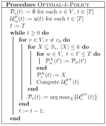
Fig. 1.Determining an optimalk-policy.

4. Determining an optimalk-policy

ByTheorem 3, finding an optimal policy is NP-hard. Note that the proof ofTheorem 2does not provide an efficient algorithm for finding an optimal policy as for a fixed nodev^{and time}^tit requires to computeU_v^P^X(t) for every subsetX ofS_v.

However, if the number of services that a policy may contain for each node–time pair is bounded by a constantk, then the problem becomes tractable. We call a policy ak-policyif|P_v(t)| ≤kfor eachv∈V,t ∈ [T]. The set ofk-policies is denoted byP_k. Ak-policyPis calledoptimalif it is optimal amongP_k, that is,U_v^P(t)≥U_v^P^′(t) for eachP^′∈P_k,v∈Vandt ∈_R. LetP_v^k(t) denote the optimalk-policy at stopv∈Vand timet ∈ [T]. The proof ofTheorem 2sheds light on the following recurrence relation between the optimal policy values:

P_v^k(t)=argmax

X⊆Sv

|X|≤k

{U_v^P^X(t)} (3)

where

P_w^X(t^′)=

{P_v^k(t^′) ift^′>^t,

X ift^′=tandw=v.

Hence we get the following recurrence relation between the optimal utility function values:

U_v^P^k(t)=max

X⊆Sv

|X|≤k T

∑

t′=_t

∑

s∈_X

⎛

⎜

⎝^U

P^k

v (t^′|s)P[D_s=t^′]∏

s′ ∈X s′ ̸=s

⎛

⎝1−

t′−₁

∑

t′′=_t

P[D_s^′ =t^′′]

⎞

⎠

⎞

⎟

⎠.

The above recurrence relations make the usage of a dynamic programming approach possible. Starting from the end of the time horizon, one can go back step-by-step in time to determine an optimalk-policy, thus giving a polynomial-time dynamic programming algorithm, calledOptimal-k-Policy, for determining an optimalk-policy.

Initially, setP_v(t)= ∅for eachv∈Vandt ∈ [T],U_v^P(t)= −∞forv̸=vdandU_v^P

d(t)=u(t), whereu(t) is the utility function given by the passenger. At a general stage of the algorithmP_v(t^′) is already defined for eachv∈Vandt^′>^t^{, and} (3)is used to determining the policy for every stopv∈Vin timet, seeFig. 1.

Recall that the maximum number of services using the same stop was denoted by∆. A very rough estimation shows that the running time of the algorithm isO(|V| ·T³·_∆^k·k²). Ifkis constant, this means to have a polynomial-time algorithm for computing an optimal policy.

5. Computational case study

In this section we compare the proposed routing method with the deterministic algorithm. The computations are based on the General Transit Feed Specification (GTFS) data of the Budapest public transport Network [7].GTFSis a common format for public transport schedules and provides for trip planning functionality, see [17]. The algorithms are implemented in C++

with heavy use of the open source LEMON graph optimization library (see [1]). The code is platform independent, the actual tests were performed on a Linux based server with a 3.50 GHz Intel Core i7-5930K CPU and 32 GB RAM.

(7)

5.1. Extending the model

For the description and analysis of the algorithm above, we have assumed a simplified model where the services were given as simple trips between two nodes without intermediate stops. For the computational case study, we use a more complex and realistic model which, according to theGTFSdata format, considers services with several trips (following each other in a prescribed order). A service has several trips consisting of several hops, hence the definition of policy must be modified accordingly. In this case, a policy is a functionP:V× [T] →2^S^×^Vsuch that if (s, w⁾∈P_v(t) then

• s∈S_v,

• w̸=vis a stop of serviceswhich is afterv^,

• (s, w^′⁾̸∈P_v(t) for each stopw^′̸=w^{of service}^s.

In the extended model, (s, w⁾∈P_v(t₀) means the following: if a passenger arrives to stopv^{at time}^t0then she is suggested to take serviceswhenever it arrives and to get off from it at stopw^.

5.2. Data preprocessing and generation of the stochastic model

In order to prepare the necessary input data, the rawGTFSdata is preprocessed in several steps. In a first step, irrelevant services are discarded so that only services working on the date of travel are considered. In a second step the list of services is filtered according to the given passenger preferences, only keeping those services that theoretically may play role in the journey. Simultaneously, a deterministic shortest path is computed between the start and the destination node as a reference solution.

Next, a probabilistic model is set up for determining arrival, departure and travel time distributions. The model may be based on the assumption of a simplified distribution (e.g., Gamma distribution for travel times), but can also take into account GTFSreal-time data and statistics obtained from real-life measurements.

5.3. Policy generation

As a starting step, an optimal deterministic solution is computed which has the highest utility in the time period defined by the user and has the latest departure time from the starting node. This is later used as a reference solution by the method to find a proper policy. Then, a dynamic programming procedure is used to determine the induced utility of being at stopv at timetfor each node and time. The length of a time interval was set to 20 s.

In the main part of the procedure, a queue of ‘active’ nodes is maintained, which is initialized with the destination node vd. At the beginning, onlyvdis marked as active. In the following iterations, assume that policies and induced utilities are computed for allv∈Vandt^′>^t. The top nodevis removed from the queue, and for each services∈S_v, timet ∈ [T]and stopw^precedingvon the route ofswe updateU_w^P(t), ^U_w^P^(t |s) according toOptimal-k-Policy, and also changeP_w(t) if necessary. If an improvement is found for some triple (s,^t, w), then stopwis pushed to the end of the queue and is marked as ‘active’. This Bellman–Ford-like algorithm computes the induced utilities for each stop and each time. The algorithm terminates when no improvement is found or an upper bound on the number of iterations is reached.

As the result is not a single route, an important question is how to represent the obtained policy. First of all, it is unnecessary to show the policy at each node, as this is only interesting for the starting node and nodes that are possibly visited during the journey. Moreover, to decrease the amount of data written out,P_v(t) is only displayed if it is not identical toP_v(t−1). The output of the model – which is a policy for each node – is further post-processed as the presence of multiple choices may result in complicated route plans. For example in case of several equally good stops it may be unclear where to take alight from a given service. The deterministic solution computed earlier is used to break ties based on latest departure times.

5.4. Test instance and results

The above procedure was applied to theGTFSdata of the Budapest public transport network. This timetable consists of 5290 stops and 135.959 services. It is not straightforward how to measure the efficiency of a policy in a stochastic environment. As the introduction of policies versus simple routes was motivated by the lack of reliability of deterministic travel plans, we measure the performance of a policy by comparing it to the usual deterministic approach. We chose an arbitrary stopvas a destination node from the map of Budapest uniformly at random, and determined the policy for each stop different fromvfor a given date and time. We considered the SOTA (Stochastic On Time Arrival) problem in all cases, that is, the utility function atvwas defined to be 1 up to a certain deadlinet_enduntil which the passenger wishes to arrive to the destination nodev, and 0 afterwards. The policies thus obtained were tested by running 500 simulations for each node.

In each instance of the simulation, the departure and travel times were assumed to follow normal distributions with expected value equal to the deterministic departure and travel times of the corresponding service, respectively. For each service, the deviations of its travel time distributions were gradually increased while following the route of the service in order to model that uncertainties between stops add up. Deviations were also changed according to time of day (light or

(8)

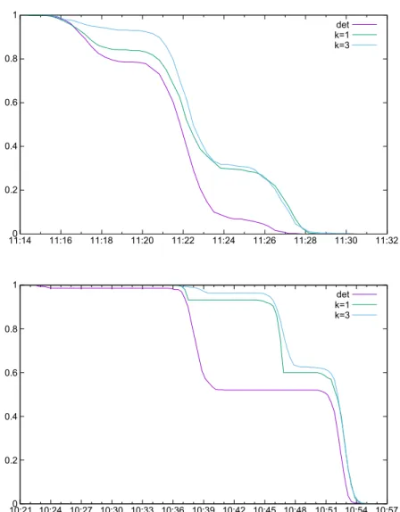
Fig. 2.Probability of arriving on time vs. departure time.

heavy traffic) and type of the service (bus, tram, subway). This method is fast and is based on reasonable assumptions on the nature of traffic, but the proposed method could be also used with historical data.

For each nodewdifferent fromvand each timet ∈ [T], we checked whether a passenger leaving from nodew^{at time} tand following either the deterministic solution or the policy succeeds to get tovin time. In both cases, for each nodew we computed the latest time instance when a user has to leave fromwin order to arrive tovin time with probability at least 90%. These values can be compared to each other for the two solutions, hence giving a benchmark for evaluating their effectiveness. In addition, it enables us to introduce the notion ofsafety marginwhich tells us how much earlier we should start compared to the latest deterministic departure so that we achieve a 90% probability of arriving in time.

Fig. 2provides illustrative examples of the achievable probability of arriving on time for different departure times from a fixed stop to a destination node. The results show that the usage of policies significantly increases the probability of arriving on time, which may be particularly useful at late departure times.

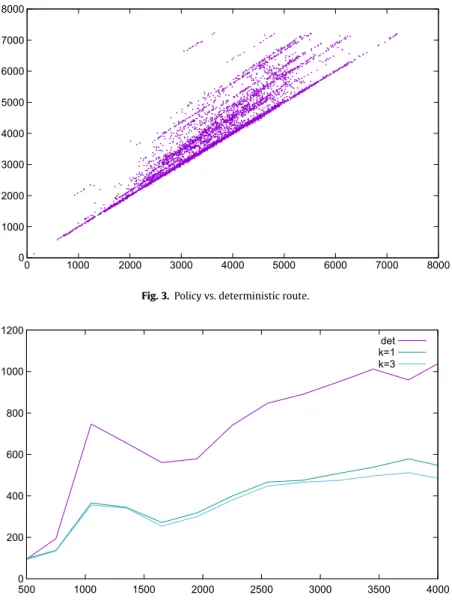
Fig. 3compares the deterministic solution and the policy for a given destination nodev. Each dot on the scatter plot represents a starting nodewdifferent fromv^{. The}^xcoordinate of a dot is the time when a passenger has to leave fromw in order to arrive tovin time with probability at least 90% when following the route of the policy, while itsycoordinate is defined similarly based on the deterministic solution. That is, dots above the liney= xcorresponds to stops from where one may leave later when following the induced policy instead of the deterministic route.

Fig. 4shows the average safety margins as a function of the deterministic travel time. The average is taken from computing the policies from all possible start positions to 4 representative destinations chosen at different parts of the city.

As we are consideringk-policies, the maximum numberkof services that the policy may contain for a given time is a parameter that has a significant effect on the efficiency of the solution. Although larger values ofkresult in better policies, it also leads to more complicated travel plans, which might discourage passengers from using the system in real applications.

(9)

Fig. 3.Policy vs. deterministic route.

Fig. 4.Average safety margin vs. deterministic travel time.

However, our simulations suggest that moderate values ofkalready lead to substantial improvements while increasingk beyond 3 leads to negligible marginal improvement. Thus, for the considered public transport system of Budapest, choosing a value ofk = 3 seems to be a reasonable compromise between solution quality and policy complexity, and we expect similar settings to perform well in other public transport networks as well.

6. Conclusion

We presented a public transport journey planning approach to cope with the typically non-deterministic public transport environment. The overall goal was to find travel policies that maximize expected utility.

At each location, a policy can encode multiple service choices, from which the traveller should take depending on which one will be arriving first. Instead of deterministic travel and arrival/departure times our model uses probability distributions, which result in a more robust, and on average more effective journey plan. Our approach can handle any passenger-defined monotone non-increasing utility functions, which allow to encode sophisticated passenger preferences beyond just ‘arriving in time’ or ‘as fast as possible’.

Acknowledgements

The authors would like to thank the anonymous reviewers for their helpful comments in improving the presentation of this work.

(10)

The first two authors were supported by the Hungarian Scientific Research Fund — OTKA, K109240. The second author was also supported by the János Bolyai Research Fellowship of the Hungarian Academy of Sciences.

References

[1]D. Balázs, A. Jüttner, P. Kovács, LEMON–an open source C++ graph template library, Electron. Notes Theor. Comput. Sci. 264 (5) (2011) 23–45.

http://lemon.cs.elte.hu.

[2]J.L. Bander, C.C. White, A heuristic search approach for a nonstationary stochastic shortest path problem with terminal cost, Transp. Sci. 36 (2) (2002) 218–230.

[3] R. Bellman, On a routing problem, Technical report, DTIC Document.

[4] K. Bérczi, A. Jüttner, M. Korom, M. Laumanns, T. Nonner, J. Szabó, Stochastic route planning in public transport, U.S. Patent No US9482542 B2, Publication date Nov 1, 2016.

[5]K. Bérczi, A. Jüttner, M. Laumanns, J. Szabó, Stochastic route planning in public transport, Transp. Res. Proc. 27 (2017) 1080–1087.

[6] A. Botea, E. Nikolova, M. Berlingerio, Multi-modal journey planning in the presence of uncertainty, in: Proceedings of the International Conference on Automated Planning and Scheduling ICAPS-13, 2013, pp. 20–28.

[7] Budapest Közlekedési Központ, Gtfs developer info,http://www.bkk.hu/en/developers/.

[8]J. Dibbelt, B. Strasser, D. Wagner, Delay-robust journeys in timetable networks with minimum expected arrival time, in: Stefan Funke, Matúš Mihalák (Eds.), 14th Workshop on Algorithmic Approaches for Transportation Modelling, Optimization, and Systems, in: OpenAccess Series in Informatics (OASIcs), vol. 42, 2014, pp. 1–14.

[9]E.W. Dijkstra, A note on two problems in connexion with graphs, Numer. Math. 1 (1) (1959) 269–271.

[10]Y. Fan, R.E. Kalaba, J.E. Moore II, Arriving on time, J. Optim. Theory Appl. 127 (3) (2005) 497–513.

[11]Y. Fan, Y. Nie, Arriving-on-time problem: discrete algorithm that ensures convergence, Transp. Res. Record: J. Transp. Res. Board (1964) 193–200.

[12]Y. Fan, Y. Nie, Optimal routing for maximizing the travel time reliability, Netw. Spat. Econ. 6 (3–4) (2006) 333–344.

[13]R.W. Floyd, Algorithm 97: shortest path, Commun. ACM 5 (6) (1962) 345.

[14] L.R. Ford, Network flow theory, Technical report, DTIC Document.

[15]H. Frank, Shortest paths in probabilistic graphs, Oper. Res. 17 (4) (1969) 583–599.

[16]M.R. Garey, D.S. Johnson, Computers and Intractability: A Guide To the Theory of NP-Completeness, 1979.

[17] GTFS, What is gtfs?https://developers.google.com/transit/gtfs/. (Accessed 6 March 2015).

[18]R.W. Hall, The fastest path through a network with random time-dependent travel times, Transp. Sci. 20 (3) (1986) 182–188.

[19]P.E. Hart, N.J. Nilsson, B. Raphael, A formal basis for the heuristic determination of minimum cost paths, IEEE Trans. Syst. Sci. Cybern. 4 (2) (1968) 100–107.

[20] D. Hoy, E. Nikolova, Approximately optimal risk-averse routing policies via adaptive discretization, in: Twenty-Ninth AAAI Conference on Artificial Intelligence, 2015, pp. 3533–3539.

[21]R.P. Loui, Optimal paths in graphs with stochastic or multidimensional weights, Commun. ACM 26 (9) (1983) 670–676.

[22]I. Murthy, S. Sarkar, Exact algorithms for the stochastic shortest path problem with a decreasing deadline utility function, European J. Oper. Res. 103 (1) (1997) 209–229.

[23] T. Nonner, Polynomial-time approximation schemes for shortest path with alternatives, in: Proceedings of the European Symposium on Algorithms ESA-12, 2012, pp. 755–765.

[24]G.H. Polychronopoulos, J.N. Tsitsiklis, Stochastic shortest path problems with recourse, Networks 27 (2) (1996) 133–143.

[25]S. Samaranayake, S. Blandin, A. Bayen, A tractable class of algorithms for reliable routing in stochastic networks, Transp. Res. C 20 (1) (2012) 199–217.

[26]S. Samaranayake, S. Blandin, A. Bayen, D. Delling, L. Liberti, Speedup techniques for the stochastic on-time arrival problem, in: 12th Workshop on Algorithmic Approaches for Transportation Modelling, Optimization, and Systems, in: OpenAccess Series in Informatics (OASIcs), vol. 25, Schloss Dagstuhl–Leibniz-Zentrum fuer Informatik, 2012, pp. 83–96.

[27]L. Yang, X. Zhou, Constraint reformulation and a Lagrangian relaxation-based solution algorithm for a least expected time path problem, Transp. Res.

B 59 (2014) 22–44.