Journal of Computational and Applied Mathematics

Contents lists available atScienceDirect

Journal of Computational and Applied Mathematics

journal homepage:www.elsevier.com/locate/cam

On the existence and stabilization of an upper unstable limit cycle of the damped forced pendulum

Balázs Bánhelyi

^a,∗

, Tibor Csendes

^a

, László Hatvani

^b

aUniversity of Szeged, Institute of Informatics, H-6720 Szeged, Árpád tér 2, Hungary

bUniversity of Szeged, Bolyai Institute, H-6720 Szeged, Árpád tér 2, Hungary

a r t i c l e i n f o

Article history:

Received 24 March 2019

Received in revised form 30 October 2019 Keywords:

Dynamical systems Pendulum Chaos Stabilization

a b s t r a c t

By the use of interval methods it is proven that there exists an unstable periodic solution to the damped and periodically forced pendulum around the upper equilibrium. It is also proved that this solution can be stabilized by a control which does not need the knowledge of values of the state variables but of the unstable periodic solution.

©2019 Elsevier B.V. All rights reserved.

1. Introduction

The mathematical pendulum is one of the most important classical models in the theory of nonlinear oscillation. In this model a particle of massmis connected by an absolute rigid and weightless rod to a base by means of a pin joint so that the particle can move in a plane. If the particle is subject to gravity, moreover the drag and the friction at the pin joint are taken into account, then the motions of the mathematical pendulum are described by the second order differential equation

ml

ϕ

^′′

= −

mgsin

ϕ − γ

^l

ϕ

^{′ (}

ϕ ∈

_R)

,

⁽¹⁾

where the state variable

ϕ

denotes the angle between the rod of the pendulum and the direction download measured counter-clockwise; g, l, and

γ >

0 are the gravity acceleration, the length of the rod, and the damping coefficient, respectively. The lower equilibrium positions

ϕ ≡

0 mod 2

π

are stable, and the upper ones

ϕ ≡ π

^{mod 2}

π

^are unstable. It was a surprising discovery at the beginning of the last century [1,2] that the upper unstable equilibria could be stabilized by vibrating the point of suspension vertically with sufficiently large frequency. Many papers (see, e.g., [3–11]

and the references therein) have been devoted to the description of this phenomenon (see also [12–14]).

J. Hubbard [15,16] investigated the motions of the forced damped pendulum (seeFig. 1).

ml

ϕ

^′′

= −

mgsin

ϕ − γ

^l

ϕ

^′

+

Acos

ω

^{t (}

ϕ ∈

_R)

.

⁽²⁾

Considering the equation with the special parameters

x^′′

= −

sinx

−

0

.

^1x′

+

cost

,

⁽³⁾

he experienced that the behavior of numerical solutions is strongly sensitive to perturbations in the initial values at certain places of the state plain. Solutions starting from similar angles and a little bit different singular velocities can be

∗ Corresponding author.

E-mail addresses: banhelyi@inf.szte.hu(B. Bánhelyi),csendes@inf.szte.hu(T. Csendes),hatvani@math.u-szeged.hu(L. Hatvani).

https://doi.org/10.1016/j.cam.2019.112702 0377-0427/©2019 Elsevier B.V. All rights reserved.

Fig. 1. The forced damped pendulum.

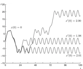
Fig. 2. Some trajectories of the forced damped pendulum.

seen inFig. 2. This phenomenon motivated him to conjecture that the system is chaotic. The chaos was exactly proved in [17], where it was also pointed out that the final reason of the chaos was the presence of an unstable 2

π

^-periodic motion around the upper equilibrium position, which bifurcated from the upper unstable periodic equilibrium. However, the existence of the unstable periodic solution was not proved, and it was not treated either how to raise the chaos. To this end it is a natural idea to stabilize the unstable periodic motion.

In Kapitsa’s procedure of the stabilization of the upper equilibrium of(1)the vertical vibration of the suspension point neutralizes the effect of the gravity. Of course, the same procedure cannot be applied to stabilize the unstable cycle of (3)since the cycle is not located in the vertical line across the suspension point. The main problem is to find the suitable vibration of the suspension point neutralizing the gravity analogous to Kapitsa’s procedure.

In this paper we prove the existence of the upper unstable periodic solution of Eq.(3)using interval methods. Then we construct a vibration of the suspension point in the plain of the motion of the pendulum(3) which stabilizes this unstable solution. This control is direct in the sense that it does not need the knowledge of values of the state variables but the unstable periodic solution. The stability of the same periodic solution guaranteed by the effect of the control is proved by interval arithmetic based tools.

2. The damped forced pendulum

2.1. The equation of motion

Eq.(3)can be rewritten into the system x^′₁

=

x₂

,

x^′₂

= −

sinx₁

−

0

.

^1x2

+

cost

,

⁽⁴⁾

wherex₁is the angle of the pendulum andx₂is the angular velocity.

2.2. The Poincaré map and periodic solutions

The following lemma says that the forced damped pendulum(4)cannot have 2

π

-periodic solutions of arbitrarily large and small initial values of the velocity.

Lemma 1. If t

↦→

(

ψ

1(t)

, ψ

2(t))is a2

π

-periodic solution of(4), then

| ψ

2(0)

| ≤

10

.

^1.

Proof. By the formula of the variation of constants (see, e.g., [18]) we have

ψ

2(t)

=

e^−0.1t

ψ

2(0)

−

e^−0.1t

∫ t

0

e^0.1s(sin

ψ

1(s)

−

coss) ds (t

∈

_R)

,

therefore

(e^0.1·2π

−

1)

ψ

2(0)

= −

∫ 2π 0

e^0.1s(sin

ψ

1(s)

−

coss) ds

.

⁽⁵⁾

Integration and the Wallis formula

∫

e^axcosbxdx

=

^e

ax

a²

+

b²

(

^bsinbx

+

acosbx

) +

const.

yield the estimate

⏐

⏐

⏐

⏐

∫ 2π 0

e^0.1s(sin

ψ

1(s)

−

coss) ds

⏐

⏐

⏐

⏐

≤

(

e^0.1·2π

−

1) (

10

+

⁰

.

¹ 1

.

⁰¹

)

.

⁽⁶⁾

From(5)and(6)we obtain the assertion. _□

Definition 1. Consider a system of ordinary differential equations

x^′

=

f(t

,

^x)

,

⁽⁷⁾

wheref

:

_R

×

_Rⁿ

→

_Rⁿ is continuous, 2

π

-periodic with respect tot and differentiable with respect tox;nis a natural number. Lett

↦→

x(t

;

t₀

,

ξ) denote the solution of(7)satisfying the initial conditionx(t₀

;

t₀

,

ξ⁾

=

ξ^{. The map}

P

:

_Rⁿ

→

_Rⁿ

,

^P(p)

=

x(2

π ;

0

,

^p) is called thePoincaré mapbelonging to Eq.(7).

In order to prove chaos, the Poincaré-map also needs to be given reliably. To do this, we apply interval arithmetic based computer assisted methods. The given proving method and the computational technique is typically well applicable to similar dynamic problems. Since this mapping cannot be represented by closed form, only one option remains, tracking the trajectory within the

[

0

,

²

π ]

time interval. The Poincaré-map of a point is given by the position of the trajectory at the t

=

2

π

moment of time. We choose VNODE (Validated Numerical ODE) [19] and INTLAB [20] due to their straight-forward and easy usage and their widely recognized performance.

The package operates based on the calculation of Taylor-series. Its strength is that it chooses the step-size automatically, therefore taking smaller steps where it is necessary. With this method, we can achieve higher accuracy. Another advantage of this package is that it can track the trajectories both forward and backward in time.

The only drawback of the program for us is that it can only give the position of the trajectory in such moments that can be represented on a computer. However, 2

π

cannot be represented on a computer in the Poincaré-map, and therefore the system of equations is used with the following modifications:

y^′₀

= π,

y^′₁

= π

^y2

,

y^′₂

= π ( −

0

.

^1y2

−

siny₁

+

cosy₀

) .

With this method, the Poincaré-map is achieved in thet

=

2 moment of time. The inverse of the Poincaré-map can be reached in att

= −

2. The values of these two functions on a two-dimensional intervalIare denoted asP(I) andP⁻¹(I).

Obviously,x(

·;

0

,

^{p) is a 2}

π

-periodic solution of(7)if and only ifpis a fixed point ofP, so if we search for periodic solutions of(7), then we have to find fixed points ofP, i.e., solutions of the equationP(p)

=

p. We will need the derivative matrixDPat a fixed pointp.

It is known [18] that the solutionx(

·;

t₀

,

ξ^{) of(7)}is differentiable with respect to the initial valuesξ, and the derivative matrixD_ξx(

·;

t₀

,

ξ) satisfies the variational system to(7)belonging to the solutionx(

·;

t₀

,

ξ^):

(D_ξx(t

;

t₀

,

ξ^))′

=

D_xf(t

,

^x(t

;

t₀

,

ξ^))Dξx(t

;

t₀

,

ξ⁾

,

^Dξx(t₀

;

t₀

,

ξ⁾

=

E

.

⁽⁸⁾ Settingξ

=

p,t₀

=

0,t

=

2

π

^{we get}

Lemma 2. Suppose that pis a fixed point ofP, and denote by

φ :

_R

→

_R^n×n the fundamental matrix of the variational differential system to(7)belonging to the2

π

-periodic solutionx(

·;

0

,

^p):

φ

^′(t)

≡

D_xf(t

,

^x(t

;

0

,

^p))

φ

^(t)

, φ

⁽⁰⁾

=

E

,

where E

∈

_R^n×nis the unit matrix. Then

DP(p)

= φ

⁽²

π

⁾

.

⁽⁹⁾

A fixed pointpof the map Pis calledstable if for every

ε >

0 there exists a

δ >

0 such that for arbitraryxwith

∥

x

−

p

∥ < δ

^{we have}

∥

P^k(x)

−

p

∥ < ε

^{for allk}

∈

_N, where

∥ · ∥

denotes an arbitrary norm inRⁿandP^kis thekth iterate ofP. A fixed point isunstableif it is not stable.

Theorem 1. There exists an unstable fixed point of the Poincaré mapPin the interval I₁

:= [

2

.

⁶³⁴²⁷²

,

²

.

⁶³⁴²⁷⁴

] × [

0

.

^02604294

,

⁰

.

^02604485

] ⊂

_R²

.

In other words, there exists a point

ξ

in this interval such that the solutionx(

·;

0

, ξ

^)of(4)is2

π

-periodic and unstable.

Proof. For finding periodic points, a simple and reliable Branch-and-Bound method was used [21]. The area of search is the initial interval

(x

,

^x′)

∈

[0

,

²

π

^]

×

[

−

10

.

¹

,

¹⁰

.

^1]

.

The B&B method generates two-dimensional intervals I_i from the initial interval to which either of the following statements is true: either theI_i interval does not have a common point with at least one ofP(I_i) andP⁻¹(I_i), or theI_i interval is small (the size is set by the user), and it has common points with bothP(I_i) andP⁻¹(I_i).

The periodic points can only lie in an interval of the second type. In the next step, intervals from this group having common points are merged into bigger intervals. This process is repeated until only pointwise disjunct intervals remain.

The number of these remaining intervals is likely equal to the number of periodic points of the system, and guaranteed bounding is achieved for all of them. In our case, only two disjoint two-dimensional intervals were found:

I₁

= [

2

.

⁶³⁴²⁷²

,

²

.

⁶³⁴²⁷⁴

] × [

0

.

^02604294

,

⁰

.

^02604485

] ,

⁽¹⁰⁾

I₂

= [

4

.

²³⁶⁸⁹³

,

⁴

.

²³⁶⁸⁹⁴

] × [

0

.

^3926964

,

⁰

.

^3926973

] .

⁽¹¹⁾

Computer simulations suggest that the first interval may contain an unstable fixed point. At the time being we only know that if there are fixed points in

[

0

,

²

π ] ×

_R, then they are contained in the two intervals above. We prove simultaneously thatI₁contains a fixed point and that the fixed point is unstable.

Consider the variational systems to(4)belonging to the solutions starting from (

ξ

1

, ξ

2)

∈

I₁: z^′₁

=

z₂

,

z^′₂

= −

sinz₁

−

0

.

^1z2

+

cost

,

^z1(0)

= ξ

1

,

^z2(0)

= ξ

2

;

z^′₃

=

z₄

,

z^′₄

= −

cosz₁(t

;

0

, ξ

1

, ξ

2)z₃

−

0

.

^1z4

.

(12)

Let

φ

⁽

·; ξ

^{) (}

φ

⁽⁰

; ξ

⁾

=

E) denote the fundamental matrix of the system of the two last equations of(12). We determined the matrix reliably by INTLAB:

φ

⁽²

π ;

(x

,

^x′)1)

=

(

[

169

.

634765210320

,

¹⁶⁹

.

640780599679

] [

168

.

790375683430

,

¹⁶⁸

.

796219219783

] [

152

.

951345297963

,

¹⁵²

.

974187177693

] [

152

.

193115985856

,

¹⁵²

.

215775203093

]

)

,

and generated guaranteed bounding intervals for the eigenvalues

λ

^1,

λ

²of this matrix by the Eig command of INTLAB:

λ

¹

∈ [

321

.

826237684765

,

³²¹

.

854884155379

] ,

λ

²

∈ [−

0

.

01311647583255

,

⁰

.

01643163463737

] .

⁽¹³⁾

If we solve the eigenvalue equation directly, we obtain a more precise result:

λ

¹1

∈ [

321

.

⁸³⁶³

,

³²¹

.

⁸³⁶⁸

] , λ

²₁

∈ [

0

.

⁰⁰¹⁴²¹

,

⁰

.

⁰⁰¹⁸⁹⁴

] .

By(9)this shows thatI₁may only contain unstable fixed points. It just remains to prove thatI₁does contain a fixed point, which will be done by the Miranda–Vrahatis theorem [22]. Define the map

F

:

_R²

→

_R²

,

^F(p)

:=

P(p)

−

p

.

Thenpis a fixed point ofP if and only ifF(p)

=

0. The Miranda–Vrahatis theorem says that if the components ofF in an appropriate decomposition are of opposite signs along the opposite parallel sides of a parallelogram in the plane, then this parallelogram contains at least one solution of the equationF(p)

=

0. It is natural to guess that one needs to decomposeF into the directions of the eigenvectors ofF, i.e., ofP. With the similar technique that was applied in [21]

we determined the parallelogram with center (2

.

⁶³⁴²⁷³

;

0

.

0260435). We searched for the directions and lengths of the

Fig. 3. The region of attraction of stable periodic solutions.

sides of the parallelogram as parameters to be optimized. We applied the objective function form as it was used in [21].

We obtained parallelograms whose sides have the directions u

:=

(0

.

762635288220063

,

⁰

.

689712810960316)

;

v

:=

(

−

0

.

703207789832756

;

0

.

711758944192742)

.

⁽¹⁴⁾

The reliably generated parallelogram isABCD, where A

=

(

[

2

.

62729502528790

,

²

.

62729502528791

] ,

[

0

.

03315291430138

,

⁰

.

03315291430139

]

)

;

B

=

(

[

2

.

62724641067606

,

²

.

62724641067607

] ,

[

0

.

03310894817352

,

⁰

.

03310894817353

]

)

;

C

=

(

[

2

.

64125097471209

,

²

.

64125097471210

] ,

[

0

.

01893408569861

,

⁰

.

01893408569862

]

)

;

D

=

(

[

2

.

64129958932393

,

²

.

64129958932394

] ,

[

0

.

01897805182647

,

⁰

.

01897805182648

]

)

.

(15)

Let us decomposeF(p) defined above in the basis

{

u

,

^v

}

: F(p)

=

F_u(p)u

+

F_v(p)v

,

i.e.,F_uandF_vdenote the components of vector F in the directionsu

,

v. We have succeeded in proving that F_u(p)

>

^{0 ifp}

∈

AD

,

^Fu(p)

<

^{0 ifp}

∈

BC

;

F_v(p)

>

^{0 ifp}

∈

CD

,

^Fv(p)

<

^{0 ifp}

∈

AB

.

HereADdenotes the convex hull of the intervalsAandD; the definitions ofBC,CD, andADare analogous. This means that all conditions of the Miranda–Vrahatis theorem are satisfied; consequently, I₁ contains a fixed point p of P for x

∈ [

0

, π ]

. On the basis of the results of our B&B method (10) (11), there can be periodic points for x

∈ [

0

, π ]

in

( [

2

.

⁶³⁴²⁷²

,

²

.

⁶³⁴²⁷⁴

] , [

0

.

^02604294

,

⁰

.

^02604485

] )

. In this box if there exists a fixed point according to the eigenvalues (13)then it must be unstable. These imply thatpexists and it is an unstable fixed point. By [12, Section 28] the 2

π

^-periodic solution corresponding to the fixed pointpof Poincaré mapPis unstable if and only ifpis unstable, which completes the proof. _□

2.3. The stable periodic point

Similarly as it was done in the proof of Theorem 1, it can be shown that there exists a point (

η

1

, η

2)

∈

I₂ from which there starts a stable periodic solution. Naturally, the solutions where the first coordinate is shifted with 2

π

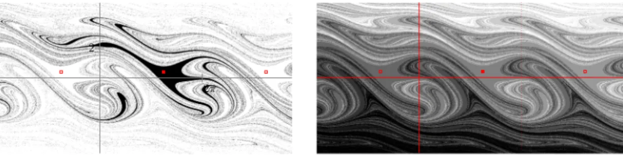
^or its multiples are behaving similarly. This solution probably bifurcated from the lower stable equilibrium state, while the unstable solution bifurcated from the upper unstable equilibrium state of the unforced pendulum.

Similarly to the unforced pendulum, the stable periodic solution has also a region of attraction, meaning that the solutions started from this region are converging to the stable periodic solutions. This region of attraction can be seen on Fig. 3(a). If this region of attraction is drawn for the other periodically shifted solutions too, then sets are formed, which are the so called Lakes of Wada [15], that is shown inFig. 3(b).

Definition 2(Lakes of Wada).The sets defined in theRⁿspace have the property of the Lakes of Wada, if a mutual boundary point of any two sets is the boundary point of every other set too.

In other words, no matter how closely a boundary is examined, all of the defined sets will appear there. In our case it means that near these boundary points all the region of attractions of the periodic solutions appear. Therefore moving away from these points arbitrarily slightly any periodic solution can be reached, which will naturally differ only in the number of previous turns.

Not all the points of the (x

,

^x′) space of the examined system belong to the region of attraction of any of the stable solutions (for example unstable solution), these points will be examined later.

3. Stabilization of the unstable solution

3.1. Stabilizing the upper equilibrium of the unforced pendulum

The literature describes two methods for stabilizing control. One of them is when the system is controlled based on the state of the dynamical system. This can be done either continuously or within discrete periods of time. This type of control, also called ‘‘feedback technique’’ stabilizes the desired state for a wider range of its initial states. The other method is when the control affecting the system does not depend on the current state of the dynamical system. In this case the stabilization can only be experienced on a smaller set of initial states.

As is known, the upper equilibrium state of the unforced pendulum is unstable. It is proven [13] that by moving the suspension point appropriately it can be stabilized. Such a result can be achieved by moving the suspension point with an oscillating motion with appropriate period and amplitude in vertical direction. (This system is usually called ‘‘Kapitsa pendulum" in honor of the Russian physicist, P.L. Kapitsa, who observed the discussed phenomenon for the first time.) Let the motion happen according to the law

ξ

^(t)

=

asin(pt)

,

where

ξ

denotes the coordinate of the suspension point on the vertical axis,ais the amplitude of the vertical displacement, andpis the number of displacements within 2

π

period of time. In this case the differential equation of the unforced pendulum can be written as

x^′′

=

(

−

^g l

−

^ap

2

l sin(pt) )

sinx

− γ

^x′

,

wherelis the length of the pendulum. To observe the stability the variation equation method can be used. In this case it is known that the pendulum has two equilibrium points, out of which one is stable (the lower equilibrium statex

=

0) and the other one is unstable (the upper equilibrium statex

= π

). Our investigation is focused on the upper equilibrium point as we want to stabilize it. The period of time of the equation above is 2

π/

p, so the variational system will be examined for this length. Within this time interval the periodic trajectory is known (x(t)

=

z₁(t)

≡ π =

const.), therefore the trajectory does not need to be calculated. With these remarks the variational system of differential equation can be given as

z^′₃

=

z₄

,

z^′₄

=

(g l

+

^ap

2

l sin(pt) )

z₃

− γ

^z4

.

⁽¹⁶⁾

Considering the case

γ =

0

.

^1,l

=

20, we examine how fast the suspension point must be moved, in other words, how large the parameterpshould be chosen so that the upper equilibrium statex

=

z₁

= π

is stable. To guarantee stability we use(9). We determine reliably the fundamental matrix

φ

^{, (}

φ

⁽²

π/

^p)

=

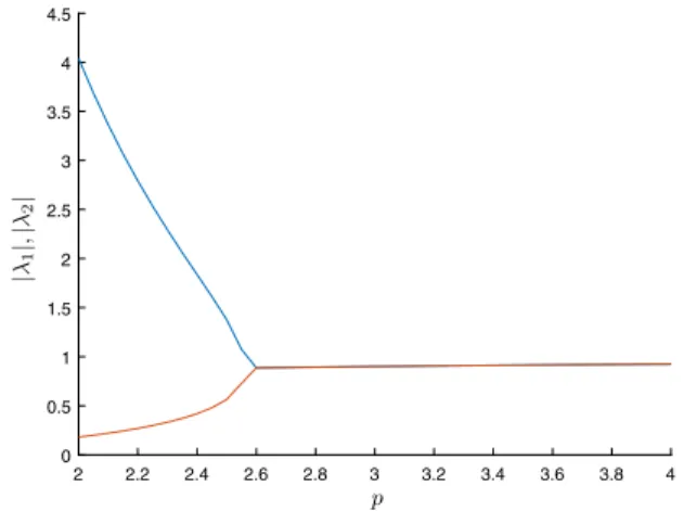
E) of(16)and its eigenvalues. To achieve stability, it is necessary and sufficient that the absolute values of the eigenvalues be less than 1.Fig. 4shows these absolute values for a constanta

=

8 and differentpparameters.

3.2. Stabilizing the upper limit cycle of the forced pendulum

Analogously to the previous method we try to stabilize the upper unstable periodic orbit, the existence of which was proved inTheorem 1. Let

ˆ

x(t) denote the angle variable of this orbit. Based on the previous results it can be anticipated that the oscillatory moving of the suspension point into the direction of_x(t

ˆ

) with acceleration of magnitude

|

ap²sin(pt)

|

with appropriate amplitudeaand frequencypwill stabilize the unstable cycle.

The unit vector in the plain pointing to the position of the suspension point is equal to (cosx(t)

ˆ ,

^sinx(t)), so the

ˆ

acceleration vector is

(u^′′(t)

, v

^′′(t))

=

(ap²sin(pt) cosx(t

ˆ

)

,

^{ap2sin(pt) sin}

ˆ

x(t))

,

⁽¹⁷⁾ and we get the control law of the moving of the suspension point by double integration. Making the choiceA

=

l

=

g,

γ =

0

.

1 again, the equation of the controlled motion has the form

x^′′

=

(

−

1

+

^u

′′(t) l

)

sinx

− v

^′′(t)

l cosx

+

cost

−

0

.

^1x′

.

⁽¹⁸⁾

Fig. 4. The absolute value of the eigenvalues as a function of the parameterp.

Theorem 2. If a

=

4and p

=

4, then the control defined by(17)stabilizes the upper unstable cycle of the damped forced pendulum(4), i.e., x

= ˆ

x(t)is a stable periodic solution of(18).

Proof. We consider the system z₁^′

=

z₂

,

z₂^′

= −

sin

(

^z1

) −

0

.

^1z2

+

cost

,

z₃^′

=

z₄

,

z₄^′

=

(

−

1

+

^ap

2

l sin(pt) cosz₁(t) )

sinz₃

−

^ap

2

l sin(pt) sinz₁(t) cosz₃

−

0

.

^1z4

+

cost

,

z₅^′

=

z₆

,

z₆^′

=

((

−

1

+

^ap

2

l sin(pt) cosz₁(t) )

cosz₃(t)

+

^ap

2

l sin(pt) sinz₁(t) sinz₃(t) )

z₅

−

0

.

^1z6

.

(19)

The variablesz₁and z₂ are identical tox₁

,

^x2 of the original differential equation of the forced damped pendulum. The purpose of the first two equations of the system is to calculate the periodic solution with which the direction of the acceleration of the suspension point can be determined. The system of the third and fourth equation forz₃

,

^z4is equivalent to the second order differential equation (18); it describes the controlled system under the influence of control(17), consequently it continuously uses the coordinatez₁(t) of the originally unstable motion yielded by the first two equations of the system. Finally we checked the stability by the fifth and sixth equation which form the variational system to the system of the third and fourth equation. We start the process with the initial values of (z₁

,

^z2) and (z₃

,

^z4) both equal to

( [

2

.

⁶³⁴²⁷²

,

²

.

⁶³⁴²⁷⁴

] , [

0

.

^02604294

,

⁰

.

^02604485

] )

^.

Settinga

=

4 andp

=

4, the two eigenvalues of the matrix obtained by the method described above for the initially unstable solution are:

λ

¹

= [−

0

.

^41408955

, −

0

.

^41383926

] + [

0

.

^60060509

,

⁰

.

^60292339

]

i

,

and

λ

²

= [−

0

.

^41408955

, −

0

.

^41383926

] − [

0

.

^60060509

,

⁰

.

^60292339

]

i

.

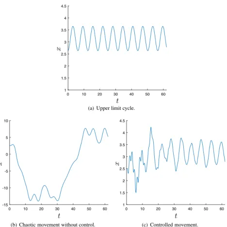
The absolute values of both multiplicators are less than one, so the originally unstable solution has become stable. □ We illuminateTheorem 2by a computer simulation.Fig. 5(b)shows the solution of the uncontrolled pendulum(4) satisfying initial conditions x₁(0)

=

2

.

^{5, x}2(0)

=

0

.

0. To demonstrate the influence of the control on this solution, in Fig. 5(c)we present the solution of(18)with the same initial condition.

Let us observe that control(17)does not depend on states of the current pendulum — neither on the speed nor the angle. Only the solution of the upper unstable trajectory is applied in these functions, which can be calculated in advance and stored. Therefore the control applied on the current problem is a kind of non-feedback techniques.

Fig. 5. Stabilization of the forced pendulum.

Acknowledgments

This research was supported by the projects ‘‘Extending the activities of the HU-MATHS-IN Hungarian Industrial and Innovation Mathematical Service Network’’ EFOP-3.6.2-16-2017-00015, and ‘‘Integrated program for training new generation of scientists in the fields of computer science’’, EFOP-3.6.3-VEKOP-16-2017-0002. Special thanks for János Horváth and Asparuh Barát for running the related computer programs.

The project has been supported by the European Union, co-funded by the European Social Fund, the János Bolyai Research Scholarship of the Hungarian Academy of Sciences, and the Unkp-18-4-Bolyai+ New National Excellence Program of the Ministry of Human Capacities, Hungary. The paper was supported by the Hungarian Scientific Research Fund (OTKA K109782).

The authors are grateful for the anonymous referees for their careful work and useful suggestions.

References

[1] A. Stephenson, On a new type of dynamical stability, Manch. Mem. 52 (1908) 1–10.

[2] P.L. Kapitsa, Dynamical stability of a pendulum when its point of suspension viberates, in: Collected Papers by P.L. Kapitsa II, Pergamon Press, Oxford, 1965.

[3] J.A. Blackburn, H.J.T. Smith, N. Gronbeck-Jensen, Stability and Hopf bifurcation in an inverted pendulum, Am. J. Phys. 60 (1992) 903–908.

[4] E. Butikov, An improved criterion for Kapitzas pendulum, J. Phys. A 44 (2011) 1–16.

[5] T. Csendes, B. Bánhelyi, L. Hatvani, Towards a computer-assisted proof for chaos in a forced damped pendulum equation, J. Comput. Appl.

Math. 199 (2007) 378–383.

[6] L. Csizmadia, L. Hatvani, An extension of the Levi-Weckesser method to the stabilization of the inverted pendulum under gravity, Meccanica 49 (2014) 1091–1100.

[7] A.M. Formalski, On the stabilization of an inverted pendulum with a fixed or moving suspension point, Dokl. Akad. Nauk 406 (2006) 175–179.

[8] M. Levi, Stability of the inverted pendulum – a topological explanation, SIAM Rev. 30 (1988) 639–644.

[9] M. Levi, Geometry of kapitsa potentials, Nonlinearity 11 (1998) 1365–1368.

[10] M. Levi, W. Weckesser, Stabilization of the inverted, linearized pendulum by high frequency vibrations, SIAM Rev. 37 (1995) 219–223.

[11] A.A. Seyranian, A.P. Seyranian, The stability of an inverted pendulum with a vibrating suspension point, J. Appl. Math. Mech. 70 (2006) 754–761.

[12] V.I. Arnold, Ordinary Differential Equations, Springer, Berlin, 2006.

[13] C. Chicone, Ordinary Differential Equations with Applications, in: Texts in Applied Mathematics, vol. 34, Springer, New York, 1999.

[14] D.R. Merkin, Introduction to the Theory of Stability, Springer-Verlag, New York, 1997.

[15] J. Hubbard, The forced damped pendulum: chaos, complication and control, Amer. Math. Monthly 106 (1999) 741–758.

[16] J. Hubbard, B. West, Chaos and control, in: ODE Architect Companion, Wiley, New York, 1999.

[17] B. Bánhelyi, T. Csendes, B.M. Garay, L. Hatvani, A computer-assisted proof forΣ3-chaos in the forced damped pendulum equation, SIAM J. Appl.

Dyn. Syst. 7 (2008) 843–867.

[18] J.K. Hale, Ordinary Differential Equations, Wiley, New York, 1969.

[19] VNODE Package home page.http://www.cas.mcmaster.ca/nedialk/software/vnode/vnode.shtml.

[20] S.M. Rump, Intlab - interval laboratory, in: Tibor Csendes (Ed.), Developments in Reliable Computing, Kluwer Academic Publishers, Dordrecht, 1999, pp. 77–104.

[21] T. Csendes, B.M. Garay, B. Bánhelyi, A verified optimization technique to locate chaotic regions of Hénon systems, J. Global Optim. 35 (2006) 145–160.

[22] M.N. Vrahatis, A short proof and a generalization of Miranda’s existence theorem, Proc. Amer. Math. Soc. 107 (1989) 701–703.