The original published PDF available in this website:
1
https://besjournals.onlinelibrary.wiley.com/doi/abs/10.1111/1365-2664.13142
2 3
A Unified Model for Optimizing Riverscape Conservation
4 5
Tibor Erős,1,2,3* Jesse R. O’Hanley,4 István Czeglédi1 6
7
1MTA Centre for Ecological Research, Balaton Limnological Institute, Klebelsberg K. u. 3, 8
H-8237 Tihany, Hungary 9
2MTA Centre for Ecological Research, Danube Research Institute, Budapest, Hungary 10
3MTA Centre for Ecological Research, GINOP Sustainable Ecosystems Group, Tihany, 11
Hungary 12
4Kent Business School, University of Kent, Canterbury CT2 7FS, UK 13
14
*Corresponding author:
15
Balaton Limnological Institute, MTA Centre for Ecological Research, Klebelsberg K. u. 3 16
H-8237 Tihany, Hungary 17
eros.tibor@okologia.mta.hu 18
19
Running title: Optimizing riverscape conservation 20
21
Word count: Total (8298), Summary (327), Main Text (5763), Acknowledgements (79), 22
Data Accessibility (18), References (1836), Tables and Figure Legends (275) 23
No. of tables: 1 24
No. of figures: 7 25
No. of references: 69 26
27
Keywords: land use planning, ecosystem services, spatial prioritization, protected area 28
networks, river barriers, habitat fragmentation, connectivity restoration, optimization 29
Abstract 30
1. Spatial prioritization tools provide a means of finding efficient trade-offs between 31
biodiversity protection and the delivery of ecosystem services. Although a large number 32
of prioritization approaches have been proposed in the literature, most are specifically 33
designed for terrestrial systems. When applied to river ecosystems, they often fail to 34
adequately account for the essential role that landscape connectivity plays in maintaining 35
both biodiversity and ecosystem services. This is particularly true of longitudinal 36
connectivity, which in many river catchments is highly altered by the presence of dams, 37
stream-road crossings, and other artificial structures.
38
2. We propose a novel framework for coordinating river conservation and connectivity 39
restoration. As part of this, we formulate an optimization model for deciding which 40
subcatchments to designate for ecosystem services and which to include in a river 41
protected area (RPA) network, while also deciding which existing river barriers to remove 42
in order to maximize longitudinal connectivity within the RPA network. In addition to 43
constraints on the size and makeup of the RPA network, the model also considers the 44
suitability of sites for conservation, based on a biological integrity index, and connectivity 45
to multiple habitat types. We demonstrate the usefulness of our approach using a case 46
study involving four managed river catchments located in Hungary.
47
3. Results show that large increases in connectivity-weighted habitat can be achieved 48
through targeted selection of barrier removals and that the benefits of barrier removal are 49
strongly depend on RPA network size. We find that (i) highly suboptimal solutions are 50
produced if habitat conservation planning and connectivity restoration are done separately 51
and (ii) RPA acquisition provides substantially greater marginal benefits than barrier 52
removal given limited resources.
53
4. Synthesis and applications. Finding a balance between conservation and ecosystem 54
services provision should give more consideration to connectivity restoration planning, 55
especially in multi-use riverscapes. We present the first modelling framework to directly 56
integrate and optimize river conservation and connectivity restoration planning. This 57
framework can help conservation managers to account better for connectivity, resulting in 58
more effective catchment scale maintenance of biological integrity and ecosystem services 59
delivery.
60 61
Introduction 62
One of the greatest challenges facing society today is the urgent need to halt the global 63
decline of biodiversity, while maintaining the capacity of ecosystem services for human well- 64
being (Bennett et al., 2015). Various studies have investigated the complex relationship 65
between biodiversity and ecosystem services (Reyers et al., 2012; Howe et al., 2014). Ideally, 66
management actions should be designed to provide a wide range of benefits, both in terms of 67
conservation and ecosystem services (a win-win situation). Often, increased biodiversity 68
conservation can only be achieved at the loss of certain ecosystem services and vice versa (a 69
win-lose situation). This is frequently the case in heavily used, human dominated landscapes, 70
where environmental managers must make difficult choices between biodiversity and 71
ecosystem service provision (Palomo et al., 2014).
72
A potential solution to this dilemma is to try to maximize the number of win-win and decrease 73
the number of win-lose situations by using spatial prioritization to find the best trade-off 74
between biodiversity protection and the delivery of ecosystem services (Cordingley et al., 75
2016; Doody et al., 2016). Such approaches, however, are still uncommon in practice. Most 76
spatial prioritization methods focus on the delineation of ecosystem service hotspots (i.e., by 77
selecting areas that are high in value for one or sometimes multiple services), rather than 78
explore potential conflicts and synergies between biodiversity and ecosystem services 79
(Cimon-Morin et al., 2013; Schröter & Remme, 2016).
80
Looking specifically at prioritization in riverine ecosystems, a frequently neglected 81
consideration is the critical role that landscape connectivity plays in the maintenance of both 82
biodiversity and ecosystem services (Taylor et al., 1993; Mitchell et al., 2013). Rivers provide 83
a multitude of vital ecosystem services, such as water supply, navigation, hydropower, 84
fishing, and recreational opportunities (Vörösmarty et al., 2010). Many of these services are 85
dependent on basic ecosystem processes, including species movements, genetic exchange, and 86
material and energy flows, which are all strongly regulated by longitudinal connectivity. At 87
the same time, the dendritic structure of rivers makes them particularly susceptible to 88
connectivity disruption (Grant et al., 2007; Hermoso et al., 2011), which, in turn, can 89
adversely impact ecosystem integrity. Indeed, river ecosystems are among the most threatened 90
worldwide, in large part because of the presence of large numbers of dams, stream-road 91
crossings, and other hydromodifications (Dynesius & Nilsson, 1994; Januchowski-Hartley et 92
al., 2013).
93
To date, research on prioritizing river habitat protection and connectivity restoration actions 94
has progressed mostly along two separate paths. One line of enquiry concerns the 95
development of planning tools for prioritizing the repair/replacement/removal (i.e., 96
mitigation) of artificial river barriers that impede aquatic organism passage, mainly fish, using 97
graph theory and optimization techniques (Erős et al., 2011; Neeson et al., 2015; King et al., 98
2017). A separate strand of research has focused on applying reserve selection methods 99
(Moilanen et al., 2008; Newbold & Siikamäki, 2009; Linke et al., 2012, Hermoso et al., 100
2017) to the design of freshwater conservation networks. Within this latter group, 101
connectivity, when it has been considered, is incorporated in a fairly simplistic manner by 102
trying to ensure that selected areas (usually subcatchments) are spatially adjacent. In neither 103
of these two research themes has the potential presence of instream barriers and their 104
associated impacts on longitudinal connectivity been addressed together with conservation 105
planning.
106
In this study, we address this shortcoming by proposing a novel approach to systematic river 107
conservation and connectivity restoration planning. More specifically, we formulate a model 108
for jointly optimizing the selection of river protected areas and barrier removals. Given a set 109
of biodiversity elements (i.e., habitat classes) in need of conservation, the aim of the model is 110
removals, subject to lower/upper limits on the amounts of protected habitat and a cap on the 112
number of barrier removals. The model adopts a limiting factors approach, in which 113
connectivity of any given river protected area is based on the minimum level of connectivity 114
to any other habitat class. We subsequently demonstrate the usefulness of our model using a 115
case study involving four river catchments located in Hungary.
116
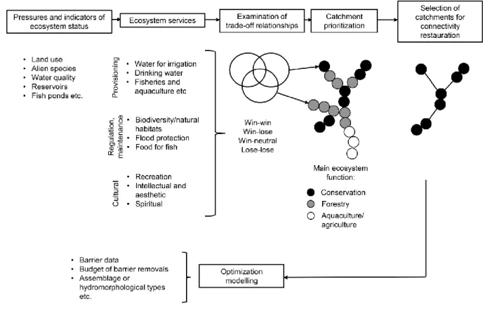
Underpinning our optimization model is a conceptual model (Fig. 1) that provides general 117
guidelines on how to systematically plan out management actions in the context of 118
biodiversity protection and ecosystem services delivery. The conceptual model combines 119
three main steps: 1) establishment of biodiversity and ecosystem service indicators; 2) 120
definition of a suitable connectivity metric; and 3) application of a spatially explicit 121
prioritization approach to efficiently allocate land use and connectivity restoration 122
management actions.
123
The first step is to develop a set of “indicators” of biodiversity and ecosystem services, 124
namely the key biological/physical elements of a system that help to maintain biodiversity and 125
ecosystem services and the various pressures that degrade ecosystem structure and function 126
(Grizetti et al., 2016; Maes et al., 2016). For example, physical and chemical water quality, 127
land use type, invasive species threats, and the presence of in-stream barriers can provide 128
useful indicators of overall ecosystem health in freshwaters (Nelson et al., 2009, Terrado et 129
al., 2016; Vital-Abarca et al., 2016).
130
The next step is to assess the role of connectivity in relation to biodiversity and ecosystem 131
services regulation in a particular system and to propose a metric that adequately describes 132
connectivity. An important consideration is the role of connectivity in producing trade-offs 133
between biodiversity and various ecosystem services. Although connectivity is critical for the 134
structuring and functioning of natural ecosystems, its importance to the delivery of ecosystem 135
services varies greatly. In stream ecosystems, for example, connectivity is critically important 136
for the dispersal of fish species, which are key components of ecosystem function and provide 137
various ecosystem services (e.g., recreational and commercial fishing, aesthetic value, see 138
Holmlund & Hammer, 1999). On the contrary, connectivity may be less important for the 139
provision of urban/agricultural water supply or for electricity, where, in fact, the damming of 140
rivers is the main way these are supplied (Auerbach et al., 2014; Grizetti et al., 2016).
141
With regard to the choice of a suitable connectivity metric, this depends on basic 142
characteristics of the system. In terrestrial applications, the adjacency/compactness of spatial 143
units makes intuitive sense (McDonnell et al., 2002; Nalle et al., 2002). In riverine systems, 144
however, connectivity between two different points in a river is dictated by the river’s flow 145
paths, making indices like the Dendritic Connectivity Index (Cote et al., 2009), which take 146
into account the passability of in-stream barriers, much more suitable (Erős et al., 2012).
147
Lastly, because resources for conservation and connectivity restoration are limited, it is 148
essential for landscape management to allocate resources in the most efficient way possible.
149
The recommendation to use a spatially explicit prioritization approach leaves two reasonable 150
alternatives: graph theory models (Erős et al., 2011) and optimization models (King et al., 151
2017). Optimization has the distinct advantage over graph theory in being prescriptive rather 152
than descriptive (King & O’Hanley, 2016), meaning that is produces a recommended course 153
of action that aims for the best allocation of limited resources to maximize benefits (i.e., 154
biggest bang for the buck). Moreover, optimization models are perfectly suited to balancing 155
multiple, potentially competing goals, thus making them ideal for driving negotiation among 156
decision makers and delivering more win-win scenarios that promote biodiversity protection 157
and ecosystem services provision.
158 159
Materials and Methods 160
Study Area 161
We selected four river catchments located in Hungary for our study (Fig. 2). These include 162
Lake Balaton (5775 km2), the Marcal River (3084 km2), the Sajó River (5545 km2), and the 163
Zagyva River (5677 km2). Catchments differ considerably in terms of the mix of land uses, 164
stream habitat type, and number of artificial barriers present (Tab. 1). The dominant land 165
cover type is agricultural (mainly arable land, vineyards to a smaller extent), but deciduous 166
forests, pastures, grasslands, and wetlands are also present. Urbanization is primarily confined 167
to small cities and villages. River habitat can be categorized into five broad types: lowland 168
river, lowland stream, highland river, highland stream, and submontane stream (Erős, 2007).
169
Biodiversity and Ecosystem Services Indicators 170
Conservation area selection methods often use simple biological diversity indicators as 171
proxies of conservation value (e.g., richness, species occurrences, endemism, species 172
composition). Rarely is attention given to the biological integrity of the ecosystem, even 173
though this may be a better indicator of a particular location’s value for conservation purposes 174
(Angermeier & Karr, 1994; Karr, 1999; Peipoch et al., 2015). According to Angermeier and 175
Karr (1994), “diversity is a collective property of system elements, integrity is a synthetic 176
property of the system.” Diversity quantifies the variety of items in the system (e.g., species 177
richness, number of functional forms), whereas integrity refers to the number of components 178
(diversity) and the processes that contribute to the continued functioning of the system in a 179
natural state. In this sense, integrity emphasizes the degree to which a system has been altered 180
from its natural (i.e., undisturbed) state (Hawkins et al., 2000; Pont et al., 2006). An 181
ecosystem with high integrity indicates that natural ecological, evolutionary, and 182
biogeographic processes are intact (Angermeier & Karr 1994; Angermeier 2000; Beechie et 183
al., 2010). Although biodiversity and biological integrity are often confused, it is important to 184
distinguish between the two, especially in the context of examining biodiversity/integrity and 185
ecosystem service relationships. For example, a reservoir created by the presence of a dam 186
may have higher biodiversity than a free-flowing stretch of river because of the occurrence of 187
both lotic and lentic species (especially waterbirds and macrophytes, which are normally less 188
abundant in undisturbed lotic areas). Stream segments impounded by a reservoir can also be 189
valuable for the provision of ecosystem services (e.g., water storage/withdrawal and 190
recreational fishing), but clearly have lower biological integrity compared to natural stream 191
segments (Beechie et al., 2010; Thorp et al., 2010; Auerbach et al., 2014).
192
We quantifid the biological integrity of stream segments and their associated subcatchments 193
using five indicators of conservation quality and naturalness. These include: 1) land use 194
intensity; 2) absolute conservation value for fish fauna; 3) relative conservation value for fish 195
fauna; 4) biological integrity of fish fauna; and 5) biological water quality. Land cover 196
categories are important indicators of ecosystem services (Grizetti et al., 2016; Maes et al., 197
2016). In this study, we used the land use index (LUI) of Böhmer et al. (2004), which 198
describes land use intensity and impact within a catchment along a gradient from natural 199
forest cover to agricultural and urban use. The index, which has been used in other studies 200
(e.g., Ligeiro et al., 2013), is calculated as follows:
201
LUI=% pasture+ 2 ×% arable land+ 4 ×% urban area
Fish assemblages are frequently used for selecting conservation areas in riverine ecosystems 202
(Filipe et al., 2004; Sowa et al., 2007). Fish are also an important focus for river connectivity 203
restoration. The absolute (ACV) and relative (RCV) conservational value of fish fauna in each 204
stream segment was determined using the index of Antal et al. (2015). To calculate ACV, 205
increasing weights were assigned to fish taxa according to their extinction risk as follows:
206
ACV = 6𝑛EW+ 5𝑛CR+ 4𝑛EN+ 3𝑛VU+ 2𝑛NT+ 𝑛LC
Here, 𝑛EW is the number of extinct species in the wild, 𝑛CR is the number of critically 207
endangered species, 𝑛EN is the number of endangered species, 𝑛VU is the number of 208
vulnerable species, 𝑛NT is the number of near threatened species, and 𝑛LC is the number of 209
least concern species (see Erős et al., 2011, Antal et al., 2015). To calculate RCV, the 210
absolute value was divided by the total number of species. Similar approaches for other 211
taxonomic groups can be found in the literature (Fattorini, 2006).
212
Biological integrity of fish assemblages (BIF) was determined using the method of Sály and 213
Erős (2016). BIF quantifies the degree of alteration of fish assemblages compared to near- 214
natural (reference) fish assemblages based on the structural and functional properties of the 215
fish fauna and their responses to different stressors (i.e., land use, water quality, and 216
hydromorphological alteration). Conceptually, BIF is similar to many other fish based biotic 217
indices (Roset et al., 2007). Additional information about how BIF was determined are 218
provided in an online appendix (see Appendix S1, Supporting Information).
219
Biological water quality (BWQ) is an integrative measure of the overall quality of the water 220
for biota. Following procedures established by the EU Water Framework Directive, biological 221
water quality was determined using the worst quality class value of five biological quality 222
indices, which measure biological water quality based on the taxonomic and functional 223
structure of benthic and water column algae, macrophytes, macroinvertebrates, and fish (Birk 224
et al., 2012). Further details about BWQ are discussed in an online appendix (see Appendix 225
S1, Supporting Information).
226
All five indices (LUI, ACV, RCV, BIF, and BWQ) were measured on a 5-point scale. An 227
aggregate biological integrity index (BII) was then determined for each stream segment by 228
taking the median of the five indices (Erős et al., 2018). Stream segments with high biological 229
integrity scores represent locations with higher biodiversity conservation value. They are also 230
essential for various regulatory (e.g., natural nursery areas) and cultural (e.g., recreational 231
hiking) ecosystem services (Grizetti et al., 2016; Vital-Abarca et al., 2016).
232
Besides the quantification of biological integrity, we also used several pressure indices to 233
identify areas within the river networks that may be better suited for alternative uses other 234
than conservation and connectivity restoration. This includes subcatchments with a high 235
urban/agricultural land use index and those where fish ponds, reservoirs, and waste water 236
treatment plants are present. Such areas are often primarily devoted to agriculture/aquaculture, 237
recreational fishing, flood control, or other ecosystem service uses and usually have low 238
biological integrity anyway (a clear win-lose situation). Based on this initial screening 239
process, all subcatchments deemed unsuitable for conservation/connectivity restoration a 240
priori were assigned a BII value of zero (Fig. 2).
241
Barrier Survey Data 242
Barrier locations were extracted from a geo-database developed by the National Water 243
Authority of Hungary. The database includes GPS referenced location information, structure 244
type (e.g., dam, road crossing, sluice), and binary passability values of potential artificial 245
barriers to fish movements. During field surveys, we further refined and updated this database 246
for the four catchments in our case study during the summer and autumn of 2016 (July to 247
November). We verified the exact location of barriers (Fig. 2), measured basic structural data, 248
and estimated upstream-downstream passability. A road network map was also used to 249
identify the location of bridges and estimate passability values for this type of barrier. In the 250
field, we determined for each barrier its height, length, and slope, type (e.g., sluice, weir, dam, 251
culvert, bridge), primary construction material (e.g., concrete, rock with concrete), 252
internal/overflow water velocity, and substrate percentages (rock, stone, gravel, sand, silt, and 253
concrete) both downstream and upstream of the barrier “wall.”
254
To estimate upstream barrier passabilities for adult cyprinids (the dominant fish species in our 255
study area), we used the rapid barrier assessment methodology described in King et al.
256
(2017). Passability represents the fraction of fish (in the range 0-1) that are able to 257
successfully negotiate a barrier in a particular direction. Each barrier assessed in the field (n = 258
703) was assigned one of four passability levels: 0 if a complete barrier to movement; 0.3 if a 259
high-impact partial barrier, passable to a small portion of fish or only for short periods of 260
time; 0.6 if a low-impact partial barrier, passable to a high portion of fish or for long periods 261
of time; and 1 if a fully passable structure (these latter structures were subsequently excluded 262
from analysis). We estimated adult cyprinid passability under both normal flow conditions 263
and bankfull width conditions. Bankfull width levels were clearly visible from the shape of 264
the channel and the location of riparian vegetation (Gordon et al., 1992). For barriers that 265
could not be surveyed because of logistical difficulties (n = 101), we assigned the median 266
passability values for a given barrier type.
267
Our surveys revealed the dominant types of barriers were stepped weirs, notched weirs (for 268
flow measurement), small fishpond dams, large reservoir dams (for irrigation and water 269
supply), and sluices. Contrary to many other countries (e.g., the US) where road culverts 270
represent the main barrier type (Januchowski-Hartley et al., 2013), such barriers are relatively 271
rare across Hungary (<1% of barriers surveyed). We also found that passability estimates 272
were very similar regardless of normal versus bankfull width flow conditions. Consequently, 273
we used passabilities under normal flow conditions for assessing river connectivity. Further, 274
given that 95% of surveyed bridges were fully passable, we excluded this type of barrier in 275
our analysis.
276
River Protection and Connectivity Optimization Model 277
To design efficiently a river protected area (RPA) network, we developed a spatial 278
optimization model to decide: 1) which subcatchments to include within the RPA network and 279
2) which barriers to mitigate (i.e., remove, repair, install with a fish pass, etc.) to maximize 280
longitudinal connectivity of the RPA network. Unlike existing optimization based methods 281
for designing RPA networks, conservation planning and connectivity restoration are made 282
simultaneously and their interactive effects were accounted for within our model. Full 283
mathematical details of the model are provided in an online appendix (see Appendix S2, 284
Supporting Information).
285
In brief, we assume that a study area is composed of one or more large, self-contained 286
catchments, with each catchment made up of potentially multiple subcatchments. Any spatial 287
resolution can be considered, from a few large subcatchments down to many small 288
subcatchments. Although a subcatchment is the main selection unit, we do not necessarily 289
assume that an entire subcatchment must be fully protected, just the river segments within a 290
selected subcatchment. The conservation value of river segments is based on a weighted 291
combination of the amount of habitat (i.e., length) and biological integrity (i.e., BII).
292
Longitudinal connectivity is quantified using a novel extension of the dendritic connectivity 293
index (DCI) proposed by Cote et al. (2009). More specifically, we evaluate DCI at the local, 294
segment-level scale (Mahlum et al. 2014) separately for each habitat type (lowland river, 295
lowland stream, highland river, highland stream, and submontane stream) and then take the 296
minimum value as an overall measure of segment connectivity. In this way, our model adopts 297
a “limiting factors” approach by focusing on the habitat type in shortest supply.
298
There are a number of constraints considered within the model for modifying the size and 299
makeup of the RPA network. These include:
300
(i) An upper limit on the size of the RPA network (i.e., the RPA network must be less 301
than or equal to some fraction of available river habitat).
302
(ii) There must be a certain mix of habitat types within the RPA network (i.e., the 303
fraction of each river habitat type must be greater than or equal to a specified 304
threshold).
305
(iii) A constraint on the number of barrier removals.
306
For our case study, we considered two barrier mitigation options: 1) full barrier removal, with 307
passability restored to 1 and 2) partial barrier removal, with passability restored to 0.5 if 308
passability currently less (Noonan et al., 2012). We assumed full removal was possible only if 309
a barrier was located in the RPA network. For a barrier outside the RPA network, only partial 310
removal was available under the presumption that the barrier was essential in providing other 311
ecosystem services (e.g., irrigation and water supply).
312
Our basic model includes separate constraints for RPA size and number of barrier removals 313
(constraints (i) and (iii) above). Given cost estimates for barrier removal and RPA land 314
acquisition, these can be easily replaced by a single budget constraint on overall cost. To 315
explore this option, a figure of €5000 per ha was used for RPA purchase (based on the cost of 316
prime agriculture land), €400k for full barrier removal, and €200k for partial barrier removal.
317
As the cost of acquiring an entire subcatchment is prohibitively expensive, we assumed that 318
only riparian areas within a 30 m distance of selected river segments had to be purchased.
319
Studies have indicated that ≥30 m buffer strips are generally sufficient to protect most aquatic 320
species (Lee et al., 2004).
321 322
Results 323
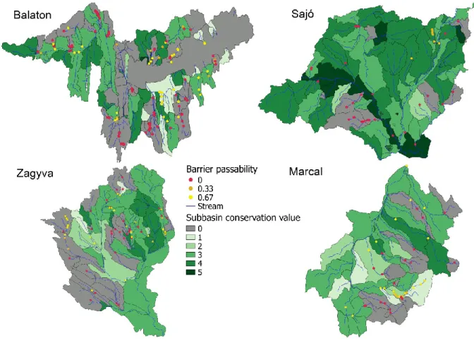
BII values varied widely both within and among the catchments (Fig. 2). In general, the 324
Balaton Catchment contained a high number of subcatchments with low or zero BII values, 325
indicating that a large part of this catchment is not ideally suited for conservation but other 326
land use functions instead. The Sajó Catchment, on the other hand, contained the highest 327
number of subcatchments with high BII values.
328
Maximum connectivity-weighted habitat for different sized RPA networks varied as a 329
function of the number of full/partial barrier removals (Fig. 3). Even with a small number of 330
barrier removals, impressive gains in connectivity-weighted habitat could be achieved. For 331
example, with a moderate sized RPA network comprising 40% of selectable river length 332
(𝜃 = 0.4), connectivity-weighted habitat increased by more than 100% (from a baseline value 333
of 1355.46 to 2813.28) when just 6 barriers were removed. In fact, strong diminishing returns 334
were observed as the number of barrier removals increased, as indicated by the concaved 335
shapes of the connectivity-weighted habitat versus barrier removal curves. Further, the 336
benefits of barrier removal were proportional to the size of the RPA network. For example, 337
for the smallest sized network encompassing 10% of selectable river length (𝜃 = 0.1), the 338
removal of 4 barriers resulted in a 26% increase in connectivity-weighted habitat. In contrast, 339
for a much larger sized network incorporating 60% of selectable river length (𝜃 = 0.6), the 340
removal of 4 barriers resulted in a 132% increase in connectivity-weighted habitat.
341
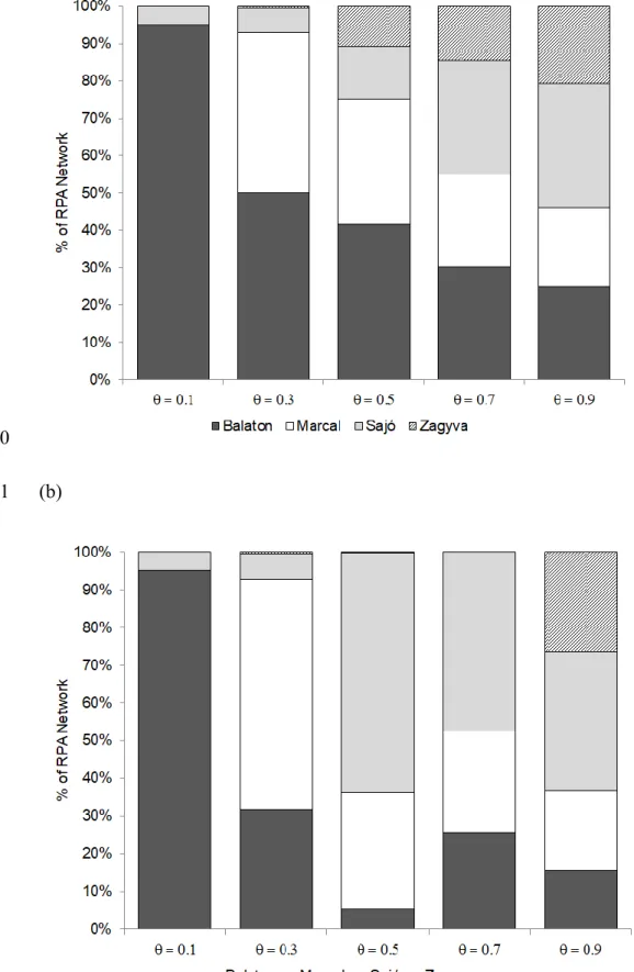
To investigate how equitably protection resources are allocated among the different river 342
catchments (Balaton, Marcal, Sajó, and Zagyva), we determined the fraction of the RPA 343
network contained in each catchment for selected values of 𝜃 given no barrier removal versus 344
an unrestricted number of barrier removals (Figs. 4 and 5). We found that both network size 345
and barrier removals strongly influenced the spatial pattern of selected subcatchments. For the 346
smallest sized reserve network (𝜃 = 0.1), protection resources are concentrated almost 347
entirely in the Balaton (95%) regardless of whether barriers can be removed or not (Figs. 4a, 348
4b, and 5a). At the other extreme, the possibility of removing barriers also does not appear to 349
dramatically alter the spatial distribution of the largest sized network (𝜃 = 0.9), with a much 350
intermediated sized networks (𝜃 = 0.3, 0.5, 0.7), the pattern is more complex. Without barrier 352
removals (Fig. 4a), the distribution of protected habitat among catchments becomes 353
progressively more balanced with increasing RPA network size. With barrier removals (Fig.
354
4b), conservation resources are directed out of the Zagyva and Balaton and into the Marcal 355
(𝜃 = 0.3) and then the Sajó (𝜃 = 0.5, 0.7; see also Fig. 5b).
356
The clear preference for concentrating conservation resources in the Balaton for the smallest 357
sized RPA network is somewhat surprising given that it is one of the most well-developed 358
areas in Hungary in terms of urbanization, aquaculture, and tourism and has a barrier density 359
(number of barriers per length of river) more than double that of any other catchment (Tab. 1).
360
Nevertheless, the Balaton is an ideal location for constructing an RPA network given very 361
limited conservation resources; it contains a significant proportion of three out of five habitats 362
types (i.e., highland stream, lowland stream, and lowland river) and a particularly favorable 363
arrangement of mostly well-connected river segments. The only way for the allocation of 364
conservation resources to dramatically shift is by modifying the basic design of the RPA 365
network (i.e., by adjusting the minimum percentage of each habitat type). Overall, the two 366
least common habitats in the four catchments are submontane stream (5.6%) and lowland 367
river (6.6%). Doubling the minimum fraction of these habitats from 80% to 160% (i.e., setting 368
𝛼 = 1.6 for these two habitat types and leaving the others at 0.8), the Balaton would account 369
for a greatly reduced, albeit still high, share (59-64%) of the 𝜃 = 0.1 sized RPA network (see 370
Appendix S3, Supporting Information). Putting very high 𝛼 weights on submontane streams 371
and highland rivers, the two least common habitat types in the Balaton, would similarly 372
reduce the amount of resources allocated to the Balaton (results not shown). These examples 373
demonstrate the flexibility of the model with regard to finding alternative solutions that meet 374
management needs. They also show that when optimizing limited conservation/restoration 375
resources, rather counterintuitive results can sometimes be obtained. For example, each 376
catchment contains roughly similar amounts of river length eligible for conservation (Tab. 1), 377
with the Balaton, Marcal, Sajó, and Zagyva contributing 22%, 19%, 33%, and 26% of the 378
total, respectively. Yet the fraction of river habitat conserved in each catchment can be very 379
far from equal depending on the size of the RPA network and the barrier removal budget.
380
We also wanted to ascertain the importance of coordinating river protection and barrier 381
removal decisions. There is considerable variability in relative connectivity-weighted habitat 382
gain when river protection decisions are made first and barrier removal decisions second (Fig.
383
6). Note that solutions for 𝑏 = 0 and 𝜃 = 1 are not considered, as these will always be 384
optimal using a two-stage approach. Results showed that river protection and restoration 385
decisions are strongly interdependent (Fig. 6). By optimizing barrier removal decisions 386
separately from river protection decisions, far less connectivity-weighted habitat is obtained, 387
with the effect exacerbated as the size of the reserve network increases. For smaller sized 388
networks (0.1 ≤ 𝜃 ≤ 0.3), 68-91% of maximum connectivity-weighted habitat can be 389
achieved (interquartile range) across all barrier removal scenarios. For moderate and large 390
sized networks (0.4 ≤ 𝜃 ≤ 0.9), however, the opportunity cost of sequential decision making 391
are much higher, with only 57-76% of the maximum being achieved (interquartile range). In 392
the worst case, just 52% of the maximum is achieved, demonstrating that highly suboptimal 393
solutions may be obtained if river protection and connectivity restoration decisions are not 394
properly coordinated.
395
Lastly, we wanted to examine the relative effectiveness of barrier mitigation against RPA land 396
purchases. To do this, we modified our basic model by first including estimates for barrier 397
removal and land purchase costs and then used a single budget for overall cost (in place of 398
separate budgets for land acquisition and barrier removal). Connectivity-weighted habitat 399
increased in a roughly linear fashion with budget (Fig. 7a). This differed from the strong 400
number of barrier removals (Fig. 3). RPA land purchases made up the majority of total spend 402
regardless of budget (Fig. 7b). At lower budgets (€5-30M), RPA land purchases accounted for 403
up to 93% of total cost. As budget increased, this percentage decreased but never below 73%
404
of total cost (at €100M). These results suggest that RPA acquisition provide substantially 405
greater marginal benefits than barrier removal, especially if resources are limited.
406
Discussion 407
In this study, we demonstrate the benefits of combining river protection and connectivity 408
restoration planning in multi-use riverscapes. As with other related work (Doody et al., 2016;
409
Zheng et al., 2016), our framework recognizes the need for a spatially informed and strategic 410
approach to the selection of different land uses for the catchment level delivery of biodiversity 411
protection and ecosystem services. Our framework is noteworthy in being the first to directly 412
incorporate connectivity restoration planning into the prioritization process using an 413
optimization based approach. Our methodology attempts to unify systematic reserve selection 414
planning with connectivity restoration planning, thus providing a powerful tool to help guide 415
protection of river ecosystems. Optimization approaches, such as ours, are specifically 416
designed to find the best allocation of limited resources to achieve one or more planning 417
goals. They are also useful for generating Pareto optimal trade-off curves, which can reveal 418
how conservation and other objectives vary with different levels of investment (Neeson et al., 419
2015).
420
Unlike some other connectivity optimization models (O’Hanley, 2011; Neeson et al. 2015), 421
our model considers the importance of maintaining access to multiple types of habitat.
422
Different riverine habitat types usually maintain different communities (Higgins et al., 2004;
423
Erős, 2007). Diversification of habitat types within an RPA network can help to ensure the 424
maximization of biodiversity (including community types). At regional scales, the common- 425
sense approach (as we have done here) is to select habitats in proportion to their natural 426
proportions within the landscape. This ensures that habitat complexity within the protected 427
area network mirrors that of the wider landscape and that a natural pattern of biodiversity is 428
maintained (Beechie et al., 2010; Thorp et al., 2010; Peipoch et al., 2015). Nevertheless, our 429
model provides decision makers with full flexibility in terms of specifying the composition of 430
an RPA network. For example, from the viewpoint of connectivity restoration for potamal fish 431
species, there is usually a preference for protecting mid- to high-order streams (King et al., 432
2017). Conversely, with future climate change likely to exert the strongest influence on 433
headwater streams (Isaak et al., 2010), it is conceivable that one would prefer to protect 434
climatically threatened low order streams. Either of these scenarios could be easily 435
accommodated for by our model (i.e., by adjusting the habitat fractions 𝛼ℎ and or the segment 436
weights 𝑤𝑠).
437
Results from our case study of four Hungarian river catchments show that impressive 438
increases in connectivity-weighted habitat can be achieved through targeted selection of 439
barrier removals, corroborating the findings of other studies (Cote et al., 2009; Branco et al., 440
2014; Neeson et al., 2015). We also observed that the benefits of barrier removal strongly 441
depend on RPA network size – for the same number of barrier removals, significantly larger 442
gains in connectivity-weighted habitat are produced as the size of the RPA network increases.
443
This is because with larger RPA networks, a much larger number of subcatchments can 444
potentially be selected, thus providing greater leeway as to which subcatchments to protect 445
and how to connect them up through barrier removal. Our results show that outcomes are 446
markedly poorer if habitat conservation and connectivity restoration decisions are made 447
separately. In the worst case, only 52% of maximum connectivity-weighted habitat is 448
achieved using a two-stage approach where conservation decisions are made first, followed by 449
barrier removal decisions. We also found that RPA land purchases provide substantially 450
greater benefits compared to barrier removals. Using a single budget for RPA acquisition and 451
barrier removals, RPA purchase always made up the bulk of spend, ranging from 73 to 93%.
452
We found that the allocation of conservation resources were sometimes very unevenly 453
distributed among different catchments. For example, for the smallest sized RPA network 454
comprising 10% of selectable river length, 95% is concentrated in Lake Balaton. Although 455
focusing on one or few target areas may make sense from a resource efficiency standpoint, it 456
can be cause for concern from a social equitability viewpoint (Halpern et al., 2013). To 457
address this, additional constraints could easily be added to our model to ensure each 458
catchments receives a certain minimum level of protection. Added justification for adopting a 459
more balanced allocation of resources might be provided if further analysis showed that 460
overall connectivity-weighted habitat only marginally decreased as a result of including these 461
supplemental constraints.
462
Our case study was framed at the multi-catchment scale, as opposed to an individual 463
catchment (Milt et al., 2017). Previous studies have shown that great efficiency is attained 464
from planning at large spatial scales (Neeson et al., 2015). From a practical standpoint, 465
however, it may be necessary to carry out planning on a catchment by catchment basis. For 466
example, our results suggest that conservation and close-to-nature forest management might 467
be the best land use functions in large parts of the Sajó Catchment, whereas agricultural land 468
use might be better suited in most part of the Zagyva and Marcal Catchments and in the 469
southern part of the Balaton Catchment. In the Sajó Catchment, forestry is already the main 470
land use function in several subcatchments and consequently, outdoor tourism (e.g., hiking, 471
recreational fishing) could be developed further in this region, while still conserving 472
biodiversity (a win-win solution). In the other catchments, where agriculture is the main land 473
use, managers should be able to easily identify those subcatchments that are the most valuable 474
for conservation, and then subsequently use our framework in the land use selection process.
475
Our modelling approach provides a set of solutions for prioritizing river conservation and 476
connectivity restoration actions based on pre-specified resources and design criteria.
477
However, in a real-world planning situation, modelling and evaluation should be done in an 478
iterative fashion, with active involvement of decision makers (Jax et al., 2013; Grizetti et al., 479
2016; McKay et al., 2017, Moody et al., 2017) in setting model parameters and performing 480
what-if analyses. For example, as our case study showed, which subcatchments are selected 481
can depend largely on the size of the RPA network and barrier removal budget. This suggests 482
that land use planners and stakeholder groups (e.g., water authorities, national park 483
authorities, fisheries groups) should ideally be involved in specifying the spatial extent of the 484
analysis, determining realistic conservation targets / barrier removal budgets, and in 485
evaluating how well conservation and ecosystem service needs are met. Their involvement 486
would be particularly useful if more reliable data could be provided on land acquisition and 487
barrier removal cost to help refine the analysis. Also, because outcomes will strongly depend 488
on the set of ecosystem services (and indicators) used in the analyses (Nelson et al., 2009), 489
involvement of planners and stakeholders groups in the earliest phases of the planning 490
procedure is essential (Jax et al., 2013).
491
Finding a balance between conservation and ecosystem services provision is a complex and 492
difficult task. There is no a single holy-grail solution that can be used to meet this need 493
(Prager et al., 2012; Terrado et al., 2016). The modelling framework presented in this paper 494
will invariably help conservation management to better account for connectivity restoration in 495
conservation planning, resulting in more effective catchment scale maintenance of biological 496
integrity and ecosystem services of riverscapes.
497 498
Authors’ Contributions 499
TE, JO’H, and IC conceived and designed the study. IC and TE collected and analyzed 500
primary research data; JO’H developed the optimization model and performed analyses of 501
model results. TE and JO’H led writing of the manuscript. All authors contributed to editing 502
manuscript drafts and gave final approval for publication.
503 504
Acknowledgements 505
This work was supported by the grants OTKA K104279 and GINOP 2.3.3-15-2016-00019.
506
We thank numerous people for help with field work and other phases of this project, but 507
especially Árpád Tóth, Rita Tóth, Péter Sály, Péter Takács, Gábor Várbíró, Andrea Zagyva, 508
and Bernadett Kern. We also thank the National Water Authority for providing us the barrier 509
dataset as well as Robert M. Hughes, an anonymous referee, and the Associate Editor for very 510
helpful comments made on an earlier draft of this paper.
511 512
Data Accessibility 513
Data available from the Dryad Digital Repository. DOI: doi:10.5061/dryad.41pj936 514
515
References 516
Angermeier, P.L. (2000) The natural imperative for biological conservation. Conservation 517
Biology, 14, 373-381.
518
Angermeier, P.L., Karr J.R. (1994) Biological integrity versus biological diversity as policy 519
directives: Protecting biotic resources. BioScience, 44, 690-697.
520
Antal, L., Harka, Á., Sallai, Z., Guti, G. (2015) TAR: Software to evaluate the conservation 521
value of fish fauna. Pisces Hungarici, 9, 71-72.
522
Auerbach, D.A., Deisenroth, D.B., McShane, R.R., McCluney, K.E., Poff N.L. (2014) 523
Beyond the concrete: Accounting for ecosystem services from free-flowing rivers.
524
Ecosystem Services, 10, 1-5.
525
Beechie, T.J., Sear, D.A., Olden, J.D., Pess, G.R., Buffington, J.M., Moir, H., Roni, P., 526
Pollock, M.M. (2010) Process-based principles for restoring river ecosystems. BioScience, 527
60, 209-222.
528
Bennett, E.M., Cramer, W., Begossi, A., et al. (2015) Linking biodiversity, ecosystem 529
services, and human well-being: Three challenges for designing research for sustainability.
530
Current Opinion in Environmental Sustainability, 14, 76-85.
531
Birk S, Bonne W, Borja A, Brucet S, Courrat A, Poikane S, et al. (2012) Three hundred ways 532
to assess Europe's surface waters: an almost complete overview of biological methods to 533
implement the Water Framework Directive. Ecological Indicators, 18, 31-41.
534
Böhmer, J., Rawer-Jost, C., Zenker, A., Meier, C., Feld, C.K., Biss, R., Hering, D. (2004) 535
Assessing streams in Germany with benthic invertebrates: Development of a multimetric 536
invertebrate based assessment system. Limnologica, 34, 416-432.
537
Branco, P., Segurado, P., Santos, J. M., Ferreira, M. T. (2014) Prioritizing barrier removal to 538
improve functional connectivity of rivers. Journal of Applied Ecology, 51, 1197-1206.
539
Cimon-Morin, J., Darveau, M., Poulin, M. (2013) Fostering synergies between ecosystem 540
services and biodiversity in conservation planning: A review. Biological Conservation, 541
166, 144–154.
542
Cordingley, J.E., Newton, A.C., Rose R.C., Clarke R.T., Bullock J.M. (2016) Can landscape- 543
scale approaches to conservation management resolve biodiversity ecosystem services 544
trade-offs? Journal of Applied Ecology, 53, 96-105.
545
Cote, D., Kehler, D.G., Bourne, C., Wiersma, Y.F. (2009) A new measure of longitudinal 546
connectivity for stream networks. Landscape Ecology, 24, 101-113.
547
Doody, D.G., Withers, P.J.A., Dils, R.M., McDowell, R.W., Smith, V., McElarney, Y.R., 548
Dunbar, M., Daly, D. (2016) Optimizing land use for the delivery of catchment ecosystem 549
services. Frontiers in Ecology and the Environment, 14, 325-332.
550
Dynesius, M., Nilsson, C. (1994) Fragmentation and flow regulation of river systems in the 551
northern third of the world. Science, 266, 753-762.
552
Erős, T. (2007) Partitioning the diversity of riverine fish: The roles of habitat types and non- 553
native species. Freshwater Biology, 52, 1400-1415.
554
Erős, T., Schmera, D., Schick, R.S. (2011) Network thinking in riverscape conservation – A 555
graph-based approach. Biological Conservation, 144, 184-192.
556
Erős, T., Olden, J.D., Schick, R.S., Schmera, D., Fortin, M-J. (2012) Characterizing 557
connectivity relationships in freshwaters using patch-based graphs. Landscape Ecology, 558
27, 303-317.
559
Erős, T., O’Hanley, J.R., Czeglédi, I. (2018) Data from: A unified model for optimizing 560
riverscape conservation. Dryad Digital Repository: https://doi.org/10.5061/dryad.41pj936 561
Fattorini, S. (2006) A new method to identify important conservation areas applied to the 562
butterflies of the Aegean Islands (Greece). Animal Conservation, 9, 75-83.
563
Filipe, A.F., Marques, T.A., Seabra, S., Tiago, P., Riberio, F., Moreira da Cost, L., Cowx, 564
I.G., Collares-Pereira, M.J. (2004) Selection of priority areas for fish conservation in 565
Guadiana river basin, Iberian Peninsula. Conservation Biology, 18, 189-200.
566
Gordon, N.D., McMahon, T.A., Finlayson, B.L. (1992) Stream Hydrology: An Introduction 567
for Ecologists. Wiley, Chichester.
568
Grant E., Lowe, W., Fagan, W. (2007) Living in the branches: Population dynamics and 569
ecological processes in dendritic networks. Ecology Letters, 10, 165-175.
570
Grizetti, B., Lanzanova, D., Liquete, C., Reynaud, A., Cardoso A.C. (2016) Assessing water 571
ecosystem services for water resource management. Environmental Science & Policy, 61, 572
194-203.
573
Halpern, B.S., Klein, C.J, Brown, C.J., et al. (2013) Achieving the triple bottom line in the 574
face of inherent trade-offs among social equity, economic return, and conservation.
575
Proceedings of National Academy of Sciences, USA, 110, 6229-6234.
576
Hawkins, C.P., Norris, R.H., Hogue, J.N., Feminella, J.W. (2000) Development and 577
evaluation of predictive models for measuring the biological integrity of streams.
578
Ecological Applications, 10, 1456-1477.
579
Hermoso, V., Filipe, A.F., Segurado, P., Beja, P. (2017) Freshwater conservation in a 580
fragmented world: Dealing with barriers in a systematic planning framework. Aquatic 581
Conservation: Marine and Freshwater Ecosystems, DOI: 10.1002/aqc.2826 582
Hermoso, V., Linke, S., Prenda, J., Possingham, H.P. (2011) Addressing longitudinal 583
connectivity in the systematic conservation planning of fresh waters. Freshwater Biology, 584
56, 57-70.
585
Higgins J.A., Bryer M.T., Khoury M.L., Fitzhugh T.W. (2004) A freshwater classification 586
approach for biodiversity conservation planning. Conservation Biology 19, 432-445.
587
Holmlund, C.M., Hammer, M. (1999) Ecosystem services generated by fish populations.
588
Ecological Economics, 29, 253-258.
589
Howe, C., Suich, H., Vira, B., Mace, G.M. (2014) Creating win-wins from tradeoffs?
590
Ecosystem services for human well-being: A meta-analysis of ecosystem service tradeoffs 591
and synergies in the real world. Global Environmental Change, 28, 263-275.
592
Isaak, D. J., Luce, C. H., Rieman, B. E., Nagel, D. E., Peterson, E. E., Horan, D. L., Parkes, 593
S., Chandler, G. L. (2010) Effects of climate change and wildfire on stream temperatures 594
and salmonid thermal habitat in a mountain river network. Ecological Applications, 20, 595
1350–1371.
596
Januchowski-Hartley, S.R., McIntyre, P.B., Diebel, M., Doran, P.J., Infante, D.M., Joseph, C., 597
Allan, D.J. (2013) Restoring aquatic ecosystem connectivity requires expanding 598
inventories of both dams and road crossings. Frontiers in Ecology and the Environment, 599
11, 211-217.
600
Jax, K., Barton, D.N., Chan, K.M.A., et al. (2013) Ecosystem services and ethics. Ecological 601
Economics, 93, 260-268.
602
Karr, J.R. (1999) Defining and measuring river health. Freshwater Biology, 41, 221–234.
603
Kemp, P.S., O’Hanley, J.R. (2010) Procedures for evaluating and prioritising the removal of 604
fish passage barriers: A synthesis. Fisheries Management and Ecology, 17, 297-322.
605
King, S. & O’Hanley, J.R. (2016) Optimal fish passage barrier removal – revisited. River 606
Research and Applications, 32, 418-428.
607
King, S., O’Hanley, J.R., Newbold, L., Kemp, P.S., Diebel, M.W. (2017) A toolkit for 608
optimizing barrier mitigation actions. Journal of Applied Ecology, 54, 599-611.
609
Lee, P., Smyth, C. Boutin, S. (2004) Quantitative review of riparian buffer width guidelines 610
from Canada and the United States. Journal of Environmental Management, 70, 165-180.
611
Ligeiro, R., Hughes, R.M., Kaufmann, P.R., et al. (2013) Defining quantitative stream 612
disturbance gradients and the additive role of habitat variation to explain macroinvertebrate 613
taxa richness. Ecological Indicators, 25, 45-57.
614
Linke, S., Kennard, M.J., Hermoso, V., Olden, J.D., Stein, J., Pusey, B.J. (2012) Merging 615
connectivity rules and large-scale condition assessment improves conservation adequacy in 616
river systems. Journal of Applied Ecology, 49, 1036-1045.
617
Maes, J., Liquete, C., Teller, A., et al. (2016) An indicator framework for assessing ecosystem 618
services in support of the EU Biodiversity Strategy to 2020. Ecosystem Services, 17, 14-23.
619
McDonnell, M.D., Possingham, H.P., Ball, I.R., Cousins, E.A. (2002) Mathematical methods 620
for spatially cohesive reserve design. Environmental Modeling and Assessment, 7, 107- 621
114.
622
McKay, S.K., Cooper, A.R., Diebel, M.W., Elkins, D., Oldford, G., Roghair, C., Wieferich, 623
D. (2017) Informing watershed connectivity barrier prioritization decisions: A synthesis.
624
River Research and Applications, 33, 847-862.
625
Milt, A.W., Doran, P.J., Ferris, M.C., Moody, A.T., Neeson, T.M., McIntyre, P.B. (2017) 626
Local-scale benefits of river connectivity restoration planning beyond jurisdictional 627
boundaries. River Research and Applications, 33, 788-795.
628
Mitchell M.G.E., Bennett E.M., Gonzalez A. (2013) Linking landscape connectivity and 629
ecosystem service provision: Current knowledge and research gaps. Ecosystems, 16, 894- 630
908.
631
Moilanen, A., Leathwick, J., Elith, J. (2008) A method for spatial freshwater conservation 632
prioritization. Freshwater Biology, 53, 577-592.
633
Moody, A.T., Neeson, T.M., Milt, A., et al. (2017) Pet project or best project? Online 634
decision support tools for prioritizing barrier removals in the Great Lakes and beyond.
635
Fisheries, 42, 57-65.
636
Nalle, D.J., Arthur, J.L., Sessions, J. (2002) Designing compact and contiguous reserve 637
networks with a hybrid heuristic approach. Forest Science, 48, 59-68.
638
Neeson, T.M., Ferris, M.C., Diebel, M.W., Doran, P.J., O'Hanley, J.R., McIntyre, P.B. (2015) 639
Enhancing ecosystem restoration efficiency through spatial and temporal coordination.
640
Proceedings of the National Academy of Sciences, USA, 112, 6236-6241.
641
Nelson, E. Mendoza, G., Regetz, J., Polasky, S., Tallis, H., Cameron, D.R, et al. (2009) 642
Modeling multiple ecosystem services, biodiversity conservation, commodity production, 643
and tradeoffs at landscape scales. Frontiers in Ecology and Environment, 7, 4-11.
644
Newbold, S.C., Siikamäki, J. (2009) Prioritizing conservation activities using reserve site 645
selection methods and population viability analysis. Ecological Applications, 19, 1774- 646
1790.
647
Noonan, M., Grant, J., Jackson, C. (2012) A quantitative assessment of fish passage 648
efficiency. Fish and Fisheries, 13, 450-464.
649
O’Hanley, J.R. (2011) Open rivers: Barrier removal planning and the restoration of free- 650
flowing rivers. Journal of Environmental Management, 92, 3112-3120.
651
O’Hanley, J.R., Scaparra, M.P., Garcia, S. (2013) Probability chains: A general linearization 652
technique for modeling reliability in facility location and related problems. European 653
Journal of Operational Research, 230, 63-75.
654
Peipoch, M., Brauns, M., Hauer, F.R., Weitere, M., Valett, M.H. (2015) Ecological 655
simplification: Human influences on riverscape complexity. Bioscience, 65, 1057-1065.
656
Palomo I., Montes C., Martín-López B., González J.A., García-Llorente M, Alcorlo P., Mora 657
M.R.G (2014) Incorporating the socio-ecological approach in protected areas in the 658
Anthropocene. Bioscience, 64, 181-191.
659
Poff, N.L., Olden, J., Meritt, D.M., Pepin, D.M. (2007) Homogenization of regional river 660
dynamics by dams and global biodiversity implications. Proceedings of the National 661
Academy of Sciences, USA, 104, 5732-5737.
662
Pont, D., Hugueny B., Beier, U., Goffaux, D., Melcher, A., Noble, R., Rogers, C., Roset, N., 663
Schmutz, S. (2006) Assessing river biotic condition at a continental scale: A European 664
approach using functional metrics and fish assemblages. Journal of Applied Ecology, 43, 665
70-80.
666
Prager, K., Reed, M., Scott, A. (2012) Encouraging collaboration for the provision of 667
ecosystem services at a landscape scale – Rethinking agri-environmental payments. Land 668
Use Policy, 29, 244-249.
669
Reyers, B., Polasky, S., Tallis, H., Mooney, H.A., Larigauderie, A. (2012) Finding common 670
ground for biodiversity and ecosystem services. BioScience, 62, 503-507.
671
Roset, N., Grenouillet, G., Goffaux, D., Kestemont, P. (2007) A review of existing fish 672
assemblage indicators and methodologies. Fisheries Management and Ecology, 14, 393- 673
405.
674
Sály, P., Erős, T. (2016) Ecological assessment of running waters in Hungary: Compilation 675
of biotic indices based on fish. Pisces Hungarici, 10, 15-45.
676
Schröter, M., Remme R.P. (2016) Spatial prioritization for conserving ecosystem services:
677
Comparing hotspots with heuristic optimization. Landscape Ecology, 31, 431-450.
678
Sowa, S.P., Annis, G., Morey, M.E., Diamond, D.D. (2007) A GAP analysis and 679
comprehensive conservation strategy for riverine ecosystems of Missouri. Ecological 680
Monographs, 77, 301-334.
681
Taylor, P.D., Fahrig, L., Henein, K., Merriam, G. (1993) Connectivity is a vital element of 682
landscape structure. Oikos, 68, 571-573.
683
Terrado, M., Momblanch, A., Bardina, M., Boithias, L., Munné, A., Sabater, S., Solera, A., 684
Acuña, V. (2016) Integrating ecosystem services in river basin management plans. Journal 685
of Applied Ecology, 53, 865-875.
686
Thorp, J.H., Flotemersch, J.E., Delong, M.D., Casper, A.F. Thoms, M.C., Ballantyne, F., 687
Williams, B.S., O'Neill, B.J., Haase, C.S. (2010) Linking ecosystem services, 688
rehabilitation, and river hydrogeomorphology. BioScience, 60, 67–74.
689
Vidal-Abarca, M.R., Santos-Martín, F., Martín-López, B., Sánchez-Montoya, M.M., Suárez 690
Alonso, M.L. (2016) Exploring the capacity of Water Framework Directive indices to 691
assess ecosystem services in fluvial and riparian systems: Towards a second 692
implementation phase. Environmental Management, 57, 1139-1152.
693
Vörösmarty, C.J., McIntyre, P.B., Gessner, M.O., et al. (2010) Global threats to human water 694
security and river biodiversity. Nature, 467, 555-561.
695
Zheng H., Li Y, Robinson BE, Liu G, Ma D, Wang F, Lu F, Ouyang Z, Daily G.C. (2016) 696
Using ecosystem service trade-offs to inform water conservation policies and management 697
practices. Frontiers in Ecology and the Environment, 14, 527–532.
698
Tables 699
Tab. 1. River habitat amounts, land use percentages, and number of artificial barriers in each river catchment. For river habitat, labels SMS, 700
HLS, HLR, LLS, and LLR correspond, respectively, to submontane stream, highland stream, highland river, lowland stream, and lowland river.
701
For land use, labels ART, AG, FOR, NFOR, WET, and WB correspond, respectively, to artificial surfaces, agriculture, forest, non-forest, 702
wetland, and water bodies.
703 704
Habitat Amount (km) Land Use (%)
Catchment SMS HLS HLR LLS LLR Total ART AG FOR NFOR WET WB No. of Barriers
Balaton 0.0 321.1 49.3 189.0 37.8 597.2 6.1 44.6 27.0 5.6 2.7 13.9 138
Marcal 20.9 157.9 0.0 252.6 70.4 501.8 5.5 64.9 24.2 5.2 0.1 0.1 50
Sajó 103.7 424.8 294.0 63.0 0.0 885.5 7.2 53.4 31.3 7.7 0.3 0.1 52
Zagyva 25.7 267.4 0.0 322.8 67.3 683.3 6.6 66.2 21.1 5.5 0.3 0.3 75
All 150.3 1171.1 343.3 827.4 175.6 2667.7 6.4 56.4 25.8 6.0 1.0 4.4 315
705
Fig. 1. A general framework for prioritizing catchments for biodiversity conservation versus 706
ecosystem services and targeting connectivity restoration actions.
707
708
Fig. 2. Spatial pattern of biological integrity (BII) and distribution of artificial barriers in the 709
four case study catchments: Lake Balaton, the Marcal River, the Sajó River, and the Zagyva 710
River. BII is shown on a five-point scale, where a darker shade of green indicates higher 711
integrity. Grey colored catchments have been assigned an integrity score of zero, indicating 712
they were deemed better suited to land use functions other than conservation/connectivity 713
restoration (e.g., agriculture). Note, that fully passable barriers (i.e. where barrier passability 714
value equals 1) are not shown on the maps.
715
716
Fig. 3. Connectivity-weighted habitat versus number of barrier removals for various sized 717
river protected area (RPA) networks.
718
(a) 719
720 (b) 721
722
Fig. 4. Fraction of the RPA network in each river catchment given no barrier removal (a) and 723
726
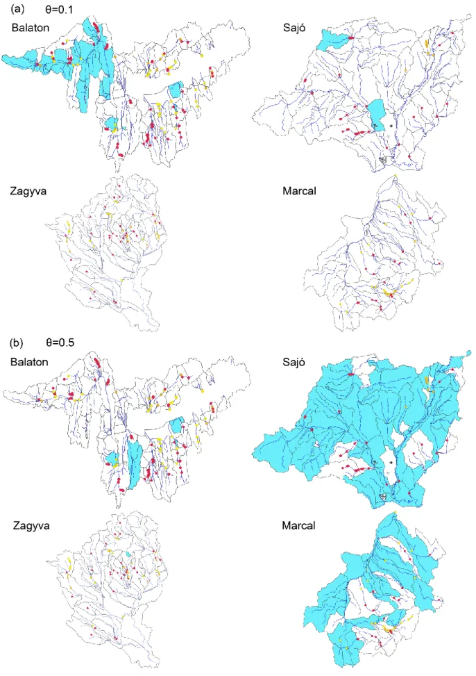
Fig. 5. Maps showing selected subcatchments for RPA networks of size 𝜃 = 0.1 (a) and 727
𝜃 = 0.5 (b) given unlimited barrier removals.
728
730 Fig. 6. Box plots showing the median, lower/upper quartiles, and minimum/maximum 731
(whiskers) amount of connectivity-weighted habitat as a percentage of maximum for various 732
RPA network sizes based on a sequential, two-stage approach to conservation and restoration 733
planning (river protection decisions made first, barrier removal decisions second).
734
(a) 735
736
(b) 737
738
Fig. 7. Connectivity-weighted habitat versus combined budget for RPA acquisition and 739
barrier removals (a) and relative spend on RPA acquisition versus barrier removal for various 740
budget amounts (b).
741