1
The original published PDF available in this website:
1
https://www.sciencedirect.com/science/article/pii/S0048969719318443?via%3Dihub 2
3
Groups of small lakes maintain larger microalgal diversity than large ones 4
5
Ágnes BOLGOVICS1*■, Viktória B-BÉRES1,2,3, Gábor VÁRBÍRÓ1,2, Eszter Ágnes 6
KRASZNAI-K1, Éva ÁCS4, Keve Tihamér KISS4, Gábor BORICS1,2■
7
8
1MTA Centre for Ecological Research, Danube Research Institute, Tisza River Department, 9
H-4026 Debrecen, Bem tér 18, Hungary 10
2MTA Centre for Ecological Research, Sustainable Ecosystems Group, H-8237 Tihany, 11
Klebelsberg Kuno u. 3, Hungary 12
3MTA-DE Lendület Functional and Restoration Ecology Research Group, H-4032 Debrecen, 13
Egyetem tér 1, Hungary 14
4MTA Centre for Ecological Research, Danube Research Institute, H-1113 Budapest, 15
Karolina út 29, Hungary 16
17
*corresponding author: Ágnes Bolgovics, e-mail address: bolgovics.agnes@okologia.mta.hu 18
■These authors contributed equally to this work.
19 20
2 Abstract
21
The question of whether one large, continuous area, or many smaller habitats maintain more 22
species is one of the most relevant questions in conservation ecology and it is referred to as 23
SLOSS (Single Large Or Several Small) dilemma in the literature. This question has not yet 24
been raised in the case of microscopic organisms, therefore we investigated whether the 25
SLOSS dilemma could apply or not to phytoplankton and benthic diatom metacommunities.
26
Benthic diatom and phytoplankton diversity in pools and ponds of different sizes (ranging 27
between 10-2 - 107 m2) was studied. Species richness of water bodies belonging the 28
neighbouring size categories was compared step by step across the whole size gradient. With 29
the exception of the compared 104–105 m2 and 105 – 106 m2 size categories, where 30
phytoplankton and benthic diatom richness values of the SL water bodies were higher than 31
that of the SS ones, diversity of several smaller (SS) sized waters was higher than that in 32
single large ones (SL) throughout the whole studied size range. The rate of the various 33
functional groups of algae, including both the benthic diatoms and phytoplankton, showed 34
remarkable changes from the smaller water bodies to large sized ones.
35
Keywords: SLOSS-dilemma, lakes, benthic diatom, phytoplankton, wide size scale 36
3 1. Introduction
37
The question of how cumulative species richness in several small habitats relates to that in 38
one large area (where cumulative area of SS is equivalent to that of SL) became known as the 39
SLOSS-debate (Single Large Or Several Small) in ecology. Several studies on the SLOSS 40
dilemma were triggered by the frightening rate of habitat fragmentations which became an 41
important issue in nature conservation (Foley et al., 2005). Since understanding the SLOSS- 42
dilemma may help to find the optimal size of nature reserves it has been studied for decades 43
by many authors since the seventies (Diamond, 1975; Wilson and Willis, 1975; Simberloff 44
and Abele, 1976). While many studies demonstrated, that from the conservational point of 45
view, several small habitats can be as valuable as a single larger-sized one (Turner and 46
Corlett, 1996; Honnay et al., 1999; Gibb and Hochuli, 2002), there are many opposing results 47
in the literature, which stress the importance of a single large habitat (Matias et al., 2010; Le 48
Roux et al., 2015). The contradictory findings of these studies indicate that this debate is still 49
unresolved (Tjørve, 2010; Rösch et al., 2015).
50
The size of the suitable habitat is largely determined by the characteristics of the species, 51
which tries to settle and establish residence. Those species that are typically generalists or 52
opportunists can easily adapt to the conditions of different-sized habitats (Gibb and Hochuli, 53
2002). High dispersal capability, that is characteristic for birds, allows them to survive in 54
small habitats in the same way as in larger ones (Lindenmayer et al., 2015). On the other 55
hand, the single large habitat ensures appropriate conditions by minimizing the extinction rate 56
(Gaz and Garcia-Boyero, 1996; Le Roux et al., 2015). Besides the specific characteristics of 57
the studied taxa, contradictory findings can also be traced back to statistical uncertainties.
58
Theoretically, the SLOSS debate is in close connection with the species-area relationship 59
(SAR). Essence of the SAR’s theory is that the species richness increases with the increasing 60
area size. This relation has been demonstrated for various organisms both on macro- (Connor 61
4
and McCoy, 1979; Tjørve, 2003; Báldi, 2008; Lindenmayer et al., 2015; Matthews et al., 62
2016) and micro-scale (Smith et al., 2005; Bolgovics et al., 2016) and now, the SAR has 63
become an accepted conceptual framework for ecological researches. Besides its theoretical 64
importance, the species-area relationship (SAR) has substantial relevance from a nature 65
conservation point of view. Although on a large spatial scale SAR can be described well by 66
power function (Arrhenius, 1921), it becomes stochastic when only a small part of the size- 67
scale is studied. It is especially true for the lower end of the size scale, where, because of the 68
so called Small Island Effect (SIE) (Triantis and Sfenthourakis, 2011; Gao and Perry, 2016), 69
diversity changes in an unpredictable way.
70
Moreover, species-area relationship can also be interpreted within the framework of the 71
metacommunity theory (Gilpin and Hanski, 1991). This theory argues that local communities 72
are linked by dispersal of many potentially interactive species, and thus create a 73
metacommunity (Leibold et al., 2004). It means that, besides the local constraints, regional 74
processes (e.g. dispersal) have pronounced influence on the composition of local 75
communities. The most common distributional patterns in meta-communities are nestedness 76
and species turnover (Baselga, 2010). Nestedness means that within a metacommunity, 77
species of some local communities are the subsets of the larger, species rich communities;
78
while species turnover is the rate of species replacement in communities, which is a reflection 79
of habitat heterogeneity (Wiens, 1974; Astorga et al., 2014). These mechanisms shape the β- 80
diversity of communities (Harrison et al., 1992), which, however, can be partitioned by the 81
appropriate statistical tools (Baselga, 2010).
82
Majority of the above mentioned findings were obtained from studies on macroscopic taxa, 83
but investigations of the SAR or the SLOSS debate on microscopic organisms may have 84
similar relevance for the understanding of the compositional structure and functioning of 85
microbial ecosystems. Diverse microbial primary producer communities in the pelagic and 86
5
benthic zone sustain diverse grazer assemblages, have an impact on their composition and 87
growth rate, and have far-reaching consequences for the structure and functioning of the 88
whole aquatic food web (Liess and Hillebrand, 2004; Striebel et al., 2012).
89
Lakes and ponds are ideal objects to investigate the SLOSS-dilemma across a large spatial 90
scale, because they can be considered as aquatic islands on a terrestrial landscape and their 91
size range may cover several orders of magnitude even within a small geographic area 92
(Dodson, 1992). These habitats provide suitable conditions for various aquatic organisms 93
from the microscopic to the macroscopic ones. Among these organisms, algae represent a 94
group which is usually characterized by high species richness and consists of taxa that are 95
relatively easy to identify. These attributes make them suitable to answer various ecologically 96
relevant questions (Soininen et al., 2016; Török et al,. 2016; Várbíró et al., 2017). In the last 97
decades, functional approaches were increasingly used in algal researches (Reynolds et al., 98
2002; Padisák et al., 2009; Rimet and Bouchez, 2012; B-Béres et al., 2016, 2017; Tapolczai et 99
al., 2016). They can provide detailed information about the ecosystem functioning and ensure 100
a deep knowledge about ecosystem vitality. Thus, they have a remarkable role in conservation 101
and environmental management (Padisák et al., 2006; Borics et al., 2007; B-Béres et al., 102
2019). In phytoplankton ecology, the functional group concept, proposed by Reynolds et al.
103
(2002), has become the most widely used classification system (Salmaso et al., 2015). Here, 104
algae and cyanobacteria are classified into more than 40 FGs based on their habitat 105
preferences and environmental tolerances (Padisák et al., 2009; Salmaso et al., 2015). In 106
diatom ecology, the use of functional classifications is based on morphological, behavioral 107
and physiological criteria (Passy, 2007; Rimet and Bouchez, 2012; Berthon et al., 2011).
108
Merging these approaches enabled the establishment of 20 combined eco-morphological 109
functional groups (CEMFGs) by B-Béres et al. (2016). The feasibility and utility of this 110
system have been studied under different environmental conditions (lowland rivers and 111
6
streams - B-Béres et al., 2017; continental saline lakes and ponds - Stenger-Kovács et al., 112
2018).
113
While the relationship between nutrients and phytoplankton biomass has been well 114
demonstrated, nutrient-diversity relationships might potentially exist only in oligotrophic or 115
oligo-mesotrophic range (Soininen and Meier, 2014), where the low nutrient concentration 116
might act as an environmental filter. In nutrient- enriched aquatic environments, causal 117
relationship between nutrient availability and species richness could not be proved (Várbíró et 118
al., 2017). In these systems the number of within-lake microhabitats has pronounced influence 119
on species diversity (Görgényi et al., 2019). Eutrophic lakes of the Carpathian Basin therefore 120
are appropriate objects to study the size-related aspects of diversity. Studying the SLOSS 121
debate on microbial aquatic organisms is not just a theoretical issue but it might also have 122
conservational relevance. In this study, we have performed an extensive analysis of the 123
SLOSS debate on a large spatial scale in Hungary using both benthic diatoms and 124
phytoplankton.
125
We addressed the following hypotheses:
126
(i) since we expect higher complexity in the larger water body categories, species 127
richness of single large (SL) water bodies will be higher than species richness of 128
several small (SS) ones 129
(ii) in accordance with the small island effect (SIE) species richness in smaller size 130
categories (10-2-102 m2) will change randomly, and clear patterns in the SLOSS 131
dilemma will not be observed, 132
(iii) since increasing complexity is expected with the increasing habitat size, this 133
complexity will result in higher number of functional groups in the case of both 134
studied group.
135 136
7 2. Material and methods
137
2.1 Study area 138
Testing the research hypotheses eutrophic pools, ponds and lakes of varying sizes were 139
selected in the whole area of Hungary (Central Europe). The area of the studied lakes covered 140
10 orders of magnitude, extending from 10-2 to 107 m2. 141
The data are partly derived from the National Hungarian Database, which contains 142
phytoplankton and phytobenthon data for shallow lakes (mean depth <3m) and ponds between 143
103-107 m2 areas. To acquire the surface area of these ponds, oxbows and other larger standing 144
water bodies we used the data of the national Hungarian database (database 1).
145
Samples belonging to the five smaller size categories (10-2-102 m2) were collected from an 146
extended area that was used as a bombing and gunnery training range between 1940 and 1990 147
and later for pasturing. This area is situated in the Hungarian Great Plain (Hungary, 47° 27' 148
00.36˝ N and 20° 59' 44.09˝), and the intensive bombing created thousands of bomb crater 149
ponds of different sizes (100-102 m2) during the decades. In this area, very small pools were 150
also created by grazing of the animals. Their sizes varied from 10-1 to 10-2 m2. To calculate the 151
area of the small pools (10-2-102 m2) at the bombing range we measured their linear 152
dimensions by a tape measure. Limnological characteristics of studied lakes can be seen in 153
Table A.1.
154
2.2 Sampling and sample processing 155
2.2.1 Diatoms 156
The sampling and sample processing of benthic diatoms were done according to international 157
standards (EN 13946, EN 14407). From shallow lakes and ponds with 103-107 m2 area, and 158
from the bomb crater ponds with 100-102 m2 area samples were collected from reed stems. At 159
those sites where macrophytes were unavailable (10-2 – 10-1 m2 size range), samples were 160
taken from the psammon. Although differences in substrata types might cause differences in 161
8
the relative abundance of the occurring elements but the species composition of psammon to 162
the harder substrates is similar (Townsend and Gell, 2005). Similar results were found by 163
Szabó et al. (2018) studying the benthic diatom flora of lakes and ponds in Hungary: They 164
found no significant differences in the composition and diversity of algal assemblages 165
collected from different substrates.
166
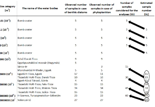
Samples from shallow lakes and ponds (103 – 107 m2 size range) were collected in the 167
growing season between 2001 and 2012, while samples from small ponds in the bombing 168
range were taken in September 2011.
169
In order to make the diatom valves clearly visible in benthic samples, 2 cm3 H2O2 were added 170
to 1 cm3 sample. In addition, a few drops of HCl were also added to remove calcium 171
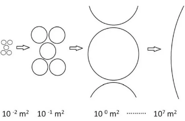
carbonate. In the next step, the samples were placed in a water bath for one day at 70 °C.
172
Finally, permanent slides were made with Cargille-Meltmount mounting medium (refractive 173
index = 1.704). Diatom species were identified with Zeiss Axioimager A2 upright microscope 174
at 1000 × magnification. Additionally, oil immersion and differential interference contrast 175
(DIC) technique were applied. A minimum of 400 valves were counted per slides.
176 177
2.2.2 Phytoplankton 178
The sampling and sample processing of phytoplankton were done according to international 179
standards (EN 16698, EN 16695, EN 15204). In the case of smaller sized pools (10-2-102 m2) 180
phytoplankton samples were taken from the middle of the pools by a plastic dish in the second 181
half of the vegetation period 2011. In the case of the shallow lakes and ponds (103-107 m2) 182
samples were collected in the vegetation period between 2001 and 2012. In these water bodies 183
more sample sites were designated in the representative points of the lakes. Samples were 184
collected from the euphotic layer with tube sampler. The euphotic layer was considered as 2.5 185
times of the Secchi depth. These subsamples were mixed in a larger plastic container, from 186
9
which 0.5 L of water was taken and fixed with formaldehyde solution (concentration of 4%) 187
and stored in darkness at 4 °C.
188
Phytoplankton samples were settled in 5 ml sedimentation chambers for 24 hours, and then 189
analysed by inverted microscopes (Utermöhl, 1958), applying 400× magnification. To 190
estimate the relative abundance of smaller algal units a minimum of 400 specimens were 191
counted. The entire area of each chamber was investigated to estimate the number of large 192
sized taxa. The list of the studied lakes and the observed number of samples are shown in 193
Table 1.
194 195
2.3 Area of the SL and SS lakes 196
Since we hypothesised that the values of the metrics used for representing the SLOSS depend 197
on the size of the water bodies, all adjacent size categories were separately compared within 198
the studied size range (10-2 - 107 m2) (Fig. 1). More precisely it means, that taxonomical and 199
functional diversities of the smaller water body category were compared to metrics of waters 200
in the next larger category.
201
In an ideal case the sum of the area of small water bodies is equal with the area of the single 202
large one. However, our database did not make possible that the area of SS lakes would be 203
equal to that of the SL one. As it is illustrated in Fig. 2, in the majority of cases, the sum of 204
the area of the SS lakes was smaller.
205
Within this smaller size range (10-2-102 m2), where we had five pools in each size category, 206
the size of SL pools was twice as large as that of the SS pools. In the larger size categories 207
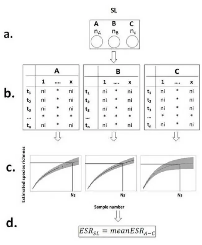
(103-107 m2) the area covered by the SS lakes also showed differences.
208 209
2.4 Species richness estimations - ESR 210
10
The observed number of species occasionally might give a biased estimate of the real species 211
richness, and the bias is mostly related to differences in the sampling effort, therefore one 212
major challenge in SLOSS studies is how to compare the species richness of the different 213
areas. Since in the smallest size categories (10-2-102 m2) single samples were collected from 214
every water body, in the case of these waters statistical richness estimations cannot be 215
applied. However, with respect to the small size of these water bodies, the sample volume/
216
habitat volume ratios were high, which increased the detectability of an individual algal unit.
217
Since higher individual detectability increases the detection of species (Buckland et al., 2011), 218
the observed number of species well represented the real species richness in these small 219
habitats. In these size categories richness values of the SS lakes were considered as the sum of 220
the observed species numbers of the 5 small pools. Species richness of the SL lake (i.e. lake in 221
one order of magnitude larger size category) was considered as the mean of the observed 222
richness values of the 5 pools belonging to the given category.
223
In the case of larger size categories (103-107 m2), data for longer time periods were available.
224
Although we had different numbers of samples from each lake in all size categories (Fig. 3A), 225
these sample numbers were sufficient to apply a more rigorous statistical comparison between 226
the richness of SL and SS lakes.
227
Since the species numbers increase with the number of the samples studied, our aim was that 228
in the pairwise comparisons between SL and SS lakes the number of samples considered 229
would be equal. To achieve this, we applied Chao’s sample-based extrapolation technique 230
(Chao et al., 2014), which is a non-asymptotic approach, that enables us to compare diversity 231
estimates by using seamless rarefaction and extrapolation (R/E) sampling curves. In the case 232
of phytoplankton, the databases usually contain species specific biomass data, which do not 233
enable the application of individual-based rarefactions. However Chao’s method is an 234
11
incidence-based technique, which considers the occurrences of species within the given 235
sample, but ignores relative abundances.
236
Increasing lake size means decreasing individual and species detectability, therefore parallel 237
with an increase in the lake size, we proposed to consider increasing sample numbers in 238
richness comparisons (Table 1). To estimate the richness in SL lakes (ESRSL) using the 239
extrapolation curves, we calculated the species richness for the proposed sample numbers for 240
each lake in the given size category (Fig. 3C), and means of these values were considered as 241
ESRSL values.
242
When estimating the species richness of SS lakes (ESRSS), as a first step, species occurrence 243
matrices of all lakes within the given size category were stacked. In the next step, applying 244
the sample numbers that were considered for calculations of ESRSL in the one order of 245
magnitude larger size category, we calculated estimated species richness of the SS lakes (Fig.
246
4C).
247
These procedures were repeated in the case of each pairwise comparison. Finally, to represent 248
the SLOSS dilemma, the quotient ESRSL/ESRSS was plotted against the area of water bodies 249
(Fig. 5).
250 251
2.5 Evaluation of functional group richness and functional redundancy 252
The observed differences between the functional group richness values of adjacent size 253
categories can be partly explained by functional differences between the compared water 254
bodies (see in subsection 2.3). These limnological and/or biological differences between water 255
bodies in adjacent size categories can result differences in the number of occurring functional 256
groups (FG) of benthic diatoms and phytoplankton (Table A.2 and A.3). Studying these 257
functional differences, taxa observed both in the benthic diatom and phytoplankton samples 258
were assigned to the appropriate FGs (Tables A.2 and A.3). Diatom species were assigned to 259
12
twenty combined eco-morphological functional groups according to B-Béres et al. (2016).
260
Functional classification of phytoplankton was based on the concept proposed by sensu 261
Reynolds et al. (2002); which was supplemented by Borics et al. (2007) and reviewed by 262
Padisák et al. (2009).
263
264
2.6 Programs used for statistical analysis 265
Rarefaction curves were drawn using the iNEXT (Hsieh et al. 2013, ver. 1.0) packages 266
available in R Studio (2012).
267 268
3. Results 269
Altogether 189 benthic diatom and 181 phytoplankton samples were collected from 36 270
different sized standing waters in Hungary. We identified 312 benthic diatom and 498 271
phytoplankton species in the samples.
272
The species richness of diatom assemblages in the SS lakes was higher at most size categories 273
(ESRSL/ESRSS values<1), except in the case of 105 m2 size range (Fig. 6 A). At the 105 m2 274
size category more species could be observed in the SL lakes than in several smaller ones 275
(ESRSL/ESRSS value>1). The ESRSL/ESRSS values showed large variation in the small size 276
categories (from 10-2 m2 to 102 m2), while they were more consistent in the case of larger 277
lakes (lake area>103 m2).
278
The results showed similar patterns in the case of the phytoplankton. The species richness of 279
SS lakes was higher in almost every size category, except in 104 m2 area size (Fig. 6 B). The 280
values showed large variation across the whole size scale, but the data showed no discernible 281
trends or regularities. In contrast to benthic diatoms where ESRSL/ESRSS ratio showed only 282
small changes in the larger lake categories, phytoplankton richness of this lake size category 283
13
was considerably smaller than that in the sum of the lakes in the adjacent smaller lake size 284
category.
285
286
3.1 Functional groups 287
The number of functional groups showed similar patterns in the case of both benthic diatoms 288
and phytoplankton. Smaller values characterized the water bodies in the 10-2 m2 to 102 m2 size 289
range, while larger ones in the 103-107 m2 range (Fig. 7 A-B, and Table A.2 and A.3).
290
Smaller differences could be observed in the larger lake categories where the number of 291
benthic diatom FGs was almost identical (~20), the phytoplankton FGs displayed a peak at 292
105 m2 range and decreased thereafter.
293
The functional redundancies of benthic diatoms (i.e. number of species within the FGs) 294
showed characteristic changes along the size gradient (Fig. 8 A and Table A.2).
295
Richness of the motile groups decreased with water body size. An opposing tendency was 296
observed in the case of high profile groups which showed increasing redundancy from 103 m2 297
to the largest size categories.
298
The ratios of the phytoplankton functional groups also differed from each other in the case of 299
smaller and larger size categories (Fig. 8B and Table A.3).
300
In small sized water bodies (10-2 m2 – 102 m2), the W1 functional group was dominant, that 301
mostly consists of euglenoid algae. In contrast to W1 group, richness of X1, N and Lo FGs 302
were higher in the larger size categories (for more information on functional groups see in 303
Table A.3).
304
305
4. Discussion 306
Our results clearly demonstrated that several small water bodies can maintain greater 307
phytoplankton and benthic diatom species richness than single large ones; thus the results did 308
14
not corroborate our first hypothesis. Considering that the aggregated areas of the several small 309
water bodies were smaller in almost each case of comparisons (Fig. 2), the results are even 310
more convincing.
311
In line with our second hypothesis the ESRSL/ESRSS values did not show any trends in the 312
case of small water bodies. Species numbers were lower and changed randomly in the smaller 313
size categories (10-2-102 m2) resulting in hectic changes in the ESRSL/ESRSS values. An 314
interesting interpretation of these results can be made in the context of the species-area 315
relationship (SAR). At large spatial scale, the SARs follow a power model (Arrhenius, 1921).
316
In contrast, the richness values change independently from the area in very small habitats, 317
resulting in unpredictable diversity patterns in these small habitats. This stochastic pattern has 318
been described as small island effect (SIE) in the literature of island biogeography (Lomolino 319
and Weiser, 2001; Triantis and Sfenthourakis, 2011). We think, that this phenomenon can 320
explain the large variations in the ESRSL/ESRSS ratio experienced in the case of small water 321
bodies.
322
Several empirical studies demonstrated that the exponent of the Arrhenius’s power-law 323
formula falls within the range of 0.1–0.5 (Lomolino, 2001), which gives a slightly asymptotic 324
character to the fitted curve. Practically, it means that drastic increase in species numbers 325
cannot be expected with increasing habitat size. Our findings are in line with this 326
phenomenon, because despite cumulative areas of SS lakes were smaller than that of the 327
single large ones, richness of SS lakes was higher than that of SL lakes. However, one 328
exception occurred both in case of phytoplankton and benthic diatoms. This can be partly 329
explained by the above mentioned methodological limitations, but other explanations should 330
also be considered. Using a large dataset, Várbíró et al. (2017) demonstrated that the shape of 331
the SAR for phytoplankton is hump shaped, having a maximum in richness about 105 -106 m2 332
range. Water bodies at this size range are exposed to moderate wind action and have an 333
15
extensive macrophyte belt; conditions which help the development of various microhabitats 334
for the phytoplankters. In large lakes, the wind induced turbulences homogenize the water 335
both horizontally and vertically creating a quasi uniform aquatic habitat. This phenomenon 336
was called the Large Lake Effect (LLE), and this seems to explain our findings that the lowest 337
values appeared in the largest size category.
338
Although dispersion ability of benthic taxa is lower than that of the planktic ones (Wetzel et 339
al., 2012), comparing to those groups where because of the obligate sexual reproduction mate 340
limitation exists (Havel and Shurin, 2004) both groups of microalgae are very good dispersers 341
(Padisák et al., 2016). Therefore, dispersal limitation is not a crucial factor affecting diversity 342
in microalgal meta-communities, instead, environmental filtering and demographic 343
stochasticity are those processes that determine the fate of colonizers in the habitats (Leibold 344
and Chase, 2017). Theoretically, the large area would benefit the colonization of habitats, but 345
size is a relative “notion” for algae, and very small habitats can satisfy the spatial needs of 346
various groups (Borics et al., 2016). The fact that ESRSS was higher than ESRSL clearly 347
highlighted that the species pool of the SS lakes cannot be considered as a subset of the SL 348
lake. Based on the logic proposed by Baselga (2010), in these situations the high species 349
turnover and the local heterogeneities maintain the compositional differences among the small 350
habitats, and contribute to the larger cumulative species and functional richness both in case 351
of phytoplankton and benthic diatoms.
352
The large within group diversity of the phytoplankton and the benthic diatoms, and the good 353
dispersal capabilities of taxa might occasionally result in species rich, but functionally 354
redundant assemblages. Therefore it is necessary to interpret the background of the SLOSS 355
dilemma at functional level. Functional richness can be a useful measure of ecosystem 356
complexity, which is determined by system attributes like amount of available resources, 357
isolation, habitat size, position of the system on the successional sequence, or random 358
16
processes e.g. colonization history and disturbances (Persson et al., 1996; Kitching, 2001;
359
Post 2002). These attributes has pronounced influence on the food-chain length, which in this 360
case can be considered as a top-down effect on the primary producers. Several field and 361
laboratory studies demonstrated that both planktic and benthic grazers prefer certain group of 362
algae (Parsons et al., 1967; Pimm and Kitching, 1987; Gresens and Lowe, 1994; Sommer, 363
1999; Kagami et al., 2002), and this preferential grazing contributes to maintain higher 364
complexity. Although an increasing complexity of water bodies could be demonstrated along 365
the size gradient (Fig. 8 A and Fig. 8 B), the functional composition of both algal groups 366
indicates, that this increasing complexity exists at the level of the whole size range (10-2 –107 367
m2). The results supported our third hypothesis, however, differences in habitat complexity 368
(number of FGs) between the adjacent size groups were not considerable, especially in the 369
case of benthic algal assemblages. An exception to this rule was the 102 –103 m2 size range, 370
where considerably higher FG richness was found in 103 m2 water bodies than in the smaller 371
ones both for benthic diatoms and phytoplankters. Typically, planktic diatoms were missing 372
from the bomb crater ponds and from the small pools, resulting in a slightly decreasing 373
complexity here. In contrast, FGs tolerating the drying up of waters (e.g. motile diatoms, or 374
codon T) (Holzinger et al., 2010; Lukács et al., 2018; B-Béres et al., 2019), were 375
characteristics in these small sized ponds and pools. The fact however, that the number of FGs 376
was almost equal in the adjacent size categories (both in the case of phytoplankton and 377
benthic diatoms) strongly implies that higher ESRSS values can be explained by the non- 378
nested nature of the species pool in the smaller water bodies, that is, identical FGs were 379
represented by different species in these waters.
380
The SLOSS debate inevitably attracted many theoretical approaches and explanations, and the 381
roots of this dilemma are deeply embedded in conservation management and landscape 382
planning. Although a popular view is, that protection of larger sized areas is better 383
17
(Tscharntke et al., 2002) investigations of different sized habitats and different animal and 384
plant groups revealed that there are arguments on “both sides of the SLOSS-debate”
385
(Tscharntke et al., 2002; Moussaoui and Auger, 2015). There is no doubt, fragmented 386
landscape is a common phenomenon worldwide, and creation of large, contiguous protected 387
areas is only rarely feasible (Gaz and Garcia-Boyero, 1996). However, as it was shown by a 388
number of studies (Tscharntke et al., 2002; Hokkanen et al., 2009; Rösch et al., 2015), in 389
certain cases, small habitats can be as valuable as larger sized areas. It is especially true for 390
small bodied organisms such as insects, snails or birds (Tscharntke et al., 2002). The results of 391
our study are not only in line with these previous findings, but demonstrate that for two 392
important microscopic aquatic groups, the higher conservational value of SS water bodies is 393
valid through the whole range of the area gradient. It is evitable, that from a practical point of 394
view, the conservation relevance of the water bodies of less than a few square meters is 395
negligible, thus, in respect to the 10-2-100 m2 size range, our results could be considered 396
theoretical curiosities. However, in Hungary, after the large river regulations of the 19th 397
century, the formerly extended bogs and marshlands disappeared almost entirely, and the 398
biota of these ecosystems now survives in the remaining small bog-pools, that mostly are not 399
larger than 102-103 m2 (Borics et al., 1998, 2003). While the Water Framework Directive 400
(2000) requires the achievement of good ecological status for all natural standing water bodies 401
larger than 50 hectares in Europe, smaller aquatic habitats do not belong under the umbrella 402
of this legislative approach. Therefore those small water bodies that are not parts of Natura 403
2000 sites are especially threatened, and need special consideration.
404
405
5. Conclusions 406
18
Results of the present study supported the view that microalgal species richness of several 407
small water bodies exceeds that of a single large one. These results are valid almost for the 408
entire scale of the area gradient, and for both phytoplankton and benthic diatoms.
409
Practical importance of these results is, that it draws attention to the fact that from a nature 410
conservation point of view, water bodies with very small areas might have relevant 411
conservational values.
412 413
6. Acknowledgement 414
We are grateful for the data provided by the Hungarian water quality monitoring network. The 415
authors were supported by the National Research, Development and Innovation Office 416
(GINOP-2.3.2-15-2016-00019) during manuscript preparation.
417
We are thankful to Tamás Bozóki for preparation of the graphical abstract.
418
419
7. Author contributions 420
ÁB wrote the manuscript. GV and EÁKK carried out the statistical analyses. VBB, ÉÁKK 421
and KTK provided data. GB raised the topic, and helped the first author during the whole 422
course of research and writing of the manuscript. All authors gave final approval for 423
publication.
424
425
8. References 426
Arrhenius, O., 1921. Species and area. J. Ecol. 9, 95–99. https://doi.org/ 10.2307/2255763.
427
Astorga, A., Death, R., Death, F., Paavola, R., Chakraborty, M., Muotka, T., 2014. Habitat 428
heterogeneity drives the geographical distribution of beta diversity: the case of New 429
Zealand stream invertebrates. Ecol. Evol. 4, 2693– 2702. https://doi.org/10.1002/ece3.1124 430
19
Báldi, A., 2008. Habitat heterogeneity overrides the species–area relationship. J. Biogeogr.
431
35, 675–681. https://doi.org/10.1111/j.1365-2699.2007.01825.x 432
Baselga, A., 2010. Partitioning the turnover and nestedness components of beta diversity.
433
Global. Ecol. Biogeogr. 19, 134-143. https://doi.org/10.1111/j.1466-8238.2009.00490.x 434
B-Béres, V., Lukács, Á., Török, P., Kókai, Zs., Novák, Z., T-Krasznai, E., Tóthmérész, B., 435
Bácsi, I. 2016. Combined eco-morphological functional groups are reliable indicators of 436
colonisation processes of benthic diatom assemblages in a lowland stream. Ecol. Ind. 64, 437
31–38. https://doi.org/10.1016/j.ecolind.2015.12.031 438
B-Béres V., Török, P., Kókai, Zs., Lukács, Á., T-Krasznai, E., Tóthmérész, B., Bácsi, I., 439
2017. Ecological background of diatom functional groups: Comparability of classification 440
systems. Ecol. Ind. 82, 183–188. https://doi.org/10.1016/j.ecolind.2017.07.007 441
B-Béres, V., Tóthmérész, B., Bácsi, I., Borics, G., Abonyi, A., Tapolczai, K., Rimet, F., 442
Bouchez, A., Várbíró, G., Török, P., 2019. Autumn drought drives functional diversity of 443
benthic diatom assemblages of continental streams. Adv. Water Resour. 126, 129–136.
444
https://doi.org/10.1016/j.advwatres.2019.02.010 445
Berthon, V., Bouchez, A., Rimet, F., 2011. Using diatom life–forms and ecological guilds to 446
assess organic pollution and trophic level in rivers: a case study of rivers in south–eastern 447
France. Hydrobiologia 673, 259–271. https://doi.org/10.1007/s10750-011-0786-1 448
Bolgovics, Á., Ács, É., Várbíró, G., Görgényi, J., Borics, G., 2016. Species area relationship 449
(SAR) for benthic diatoms: a study on aquatic islands. Hydrobiologia. 764, 91-102.
450
https://doi.org/10.1007/s10750-015-2278-1 451
Borics, G., Padisák, J., Grigorszky, I., Oldal, I., Péterfi, L.S., Momeu, L., 1998. Green algal 452
flora of the acidic bog-lake, Balata-to, SW Hungary. Biologia. 53, 457-465.
453
Borics, G., Tóthmérész, B., Grigorszky, I., Padisák, J., Várbíró, G., Szabó, S., 2003. Algal 454
assemblage types of bog-lakes in Hungary and their relation to water chemistry, 455
20
hydrological conditions and habitat diversity. In Phytoplankton and Equilibrium Concept:
456
The Ecology of Steady-State Assemblages. Springer, Dordrecht. p:145-155.
457
Borics, G., Tóthmérész, B., Várbíró, G., Grigorszky, I., Czébely, A., Görgényi, J., 2016.
458
Functional phytoplankton distribution in hypertrophic systems across water body size.
459
Hydrobiologia. 764, 81-90. https://doi.org/10.1007/s10750-015-2268-3 460
Borics, G., Várbíró, G., Grigorszky, I., Krasznai, E., Szabó, S., Kiss, K.T., 2007. A new 461
evaluation technique of potamo–plankton for the assessment of the ecological status of 462
rivers. Arch. Hidrobiol. Suppl. 17, 465–486. https://doi.org/ 10.1127/lr/17/2007/465 463
Buckland, S.T., Studeny, A.C., Magurran, A.E. and Newson, S.E., 2011. Biodiversity 464
monitoring: the relevance of detectability. in: A Magurran, A., McGill, B., (Eds.), 465
Biological Diversity: Frontiers in Measurement and Assessment. Oxford University Press, 466
pp. 25-36.
467
Chao, A., Gotelli, N.J., Hsieh, T.C., Sander, E.L., Ma, K.H., Colwell, R.K., Ellison, A.M., 468
2014. Rarefaction and extrapolation with Hill numbers: a framework for sampling and 469
estimation in species diversity studies. Ecol. Monogr. 84, 45-67.
470
https://doi.org/10.1890/13-0133.1 471
Connor, E.F., McCoy, E., 1979. The statistics and biology of the species-area relationship.
472
Am. Nat. 113, 791-833. http://www.jstor.org/stable/2460305.
473
Diamond, J.M., 1975. The island dilemma: lessons of modern biogeographic studies for the 474
design of natural reserves. Biol. Conserv. 7, 129-146. https://doi.org/10.1016/0006- 475
3207(75)90052-X 476
Dodson, S.I., 1992. Predicting Crustacean zooplankton species richness. Limnol. Oceanogr.
477
37, 848–856. https://doi.org/10.4319/lo.1992.37.4.0848 478
EC (2000) Directive 2000/60/EC of the European Parliament and of the Council of 23rd 479
October 2000 establishing a framework for Community action in the field of water policy.
480
21
Official Journal of the European Communities, 22 December, L 327/1. European 481
Commission, Brussels.
482
Fahrig, L., 2002. Effect of habitat fragmentation on the extinction threshold: a synthesis. Ecol.
483
Appl. 12, 346-353. https://doi.org/10.1890/1051-0761(2002)012[0346:EOHFOT]2.0.CO;2 484
Fahrig, L., 2003. Effects of habitat fragmentation on biodiversity. Annu. Rev. Ecol. Evol. S.
485
34, 487-515. https://doi.org/10.1146/annurev.ecolsys.34.011802.132419 486
Fischer, J., Lindenmayer, D.B., 2007. Landscape modification and habitat fragmentation: a 487
synthesis. Global. Ecol. Biogeogr. 16, 265–280. https://doi.org/10.1111/j.1466- 488
8238.2007.00287.x 489
Foley, J.A., DeFries, R., Asner, G.P., Barford, C., Bonan, G., Carpenter, S.R., Chapin, F.S., 490
Coe, M.T., Daily, G.C., Gibbs, H.K., Helkowski, J.H., Holloway, T., Howard, E.A., 491
Kucharik, C.J., Monfreda, C., Patz, J.A., Prentice, I.C., Ramankutty, N., Snyder, P.K..
492
2005. Global consequences of landuse. Science. 309, 570-574.
493
https://doi.org/10.1126/science.1111772 494
Gao, D., Perry, G., 2016. Detecting the small island effect and nestedness of herpetofauna of 495
the West Indies. Ecol. Evol. 15, 5390– 5403. https://doi.org/10.1002/ece3.2289 496
Gaz, A., Garcia-Boyero, A., 1996. The SLOSS-dilemma: a butterfly case study. Biodivers.
497
Conserv. 5, 493-502. https://doi.org/10.1007/BF00056393 498
Gibb, H., Hochuli, D.F., 2002. Habitat fragmentation in an urban environment: large and 499
small fragments support different arthropod assemblages. Biol. Conserv. 106, 91–100.
500
https://doi.org/10.1016/S0006-3207(01)00232-4 501
Gilpin, M.E., Hanski, I.A., 1991. Metapopulation dynamics: brief history and conceptual 502
domain. Biol. J. Linn. Soc. 42, 3–16. https://doi.org/10.1111/j.1095-8312.1991.tb00548.x 503
Gresens, S.E. Lowe, R.L., 1994. Periphyton patch preference in grazing chironomid larvae. J.
504
N. Am. Benthol. Soc., 13, 89–99. https://doi.org/10.2307/1467269 505
22
Görgényi, J.,Tóthmérész, B., Várbíró, G., Abonyi, A., T-Krasznai, E., B-Béres V., . Borics, 506
G., 2019. Contribution of phytoplankton functional groups to the diversity of a eutrophic 507
oxbow lake Hydrobiologia ACCEPTED in Hydrobiologia. https://doi.org/10.1007/s10750- 508
018-3878-3 509
Havel, J.E., Shurin, J.B., 2004. Mechanisms, effects, and scales of dispersal in freshwater 510
zooplankton. Limnol Oceanogr. 49, 1229-1238.
511
https://doi.org/10.4319/lo.2004.49.4_part_2.1229 512
Harrison, S., Ross, S.J., Lawton, J.H., 1992. Beta-diversity on geographic gradients in Britain.
513
J. Anim. Ecol. 61, 151–158. https://doi.org/10.2307/5518 514
Hokkanen, P.J., Kouki, J., Komonen, J., 2009. Nestedness. SLOSS and conservation networks 515
of boreal herb-rich forests. Appl. Veg. Sci. 12, 295–303. https://doi.org/10.1111/j.1654- 516
109X.2009.01031.x 517
Holzinger, A., Tschaikner, A., Remias, D., 2010. Cytoarchitecture of the desiccation-tolerant 518
green alga Zygogonium ericetorum. Protoplasma 243, 15–24. DOI 10.1007/s00709-009- 519
0048-5 520
Honnay, O., Hermy, M., Coppin, P., 1999. Effects of area, age and diversity of forest patches 521
in Belgium on plant species richness, and implications for conservation and reforestation.
522
Biol. Conserv. 87, 73–84. https://doi.org/10.1016/S0006-3207(98)00038-X 523
Hsieh, T.C., Ma, K.H., Chao, A., 2013. iNEXT online: interpolation and extrapolation 524
(Version 1.0) [Software]. Available from http://chao.stat.nthu. edu. tw/blog/software- 525
download.
526
Hylander, K., Nilsson, C., Gunnar-Jonsson, B., Göthner, T., 2005. Differences in habitat 527
quality explain nestedness in a land snail meta‐ community. Oikos. 108, 351-361.
528
https://doi.org/10.1111/j.0030-1299.2005.13400.x 529
23
Kagami, M., Yoshida, T., Gurung, T. and Urabe, J., 2002. Direct and indirect effects of 530
zooplankton on algal composition in in situ grazing experiments. Oecologia, 133(3), 356–
531
363. https://doi.org/10.1007/s00442-002-1035-0 532
Le Roux, D.S., Ikin, K., Lindenmayer, D.B., Manning, A.D., Gibbons, P., 2015. Single large 533
or several small? Applying biogeographic principles to tree-level conservation and 534
biodiversity offsets. Biol. Conserv. 191, 558–566.
535
https://doi.org/10.1016/j.biocon.2015.08.011 536
Leibold, M.A., Chase, J.M., 2017. Metacommunity ecology (Vol. 59). Princeton University 537
Press.
538
Leibold, M.A., Holyoak, M., Mouquet, N., Amarasekare, P., Chase, J.M., Hoopes, M.F., Holt, 539
R.D., Shurin, J.B., Law, R., Tilman, D., Loreau, M., Gonzalez, A., 2004. The 540
metacommunity concept: a framework for multi-scale community ecology. Ecol. Lett. 7, 541
601–613. https://doi.org/10.1111/j.1461-0248.2004.00608.x 542
Liess, A., Hillebrand, H., 2004. Invited review: direct and indirect effects in herbivore 543
periphyton interactions. Fund. Appl. Limnol. 159, 433–453. DOI: 10.1127/0003- 544
9136/2004/0159-0433 545
Lindenmayer, D.B., Wood, J., McBurney, L., Blair, D., Banks, S.C., 2015. Single large versus 546
several small: The SLOSS debate in the context of bird responses to a variable retention 547
logging experiment. Forest Ecol. Manag. 339, 1–10.
548
https://doi.org/10.1016/j.foreco.2014.11.027 549
Lomolino, M.V., Weiser, M.D., 2001. Towards a more general species–area relationship:
550
diversity on all islands, great and small. J. Biogeogr. 28, 431–445.
551
https://doi.org/10.1046/j.1365-2699.2001.00550.x 552
Lomolino, M.V., 2001. The species–area relationship: new challenges for an old pattern.
553
Prog. Phys. Geog. 25, 1–21. https://doi.org/10.1177/030913330102500101 554
24
Lukács, Á., Kókai, Zs., Török, P., Bácsi, I., Borics, G., Várbíró, G., T-Krasznai, E., 555
Tóthmérész, B., B-Béres, V., 2018. Colonisation processes in benthic algal communities 556
are well reflected by functional groups. Hydrobiologia 823, 231–245.
557
https://doi.org/10.1007/s10750-018-3711-z 558
Matias, M.G., Underwood, A.J., Hochuli, D.F., Coleman, R.A., 2010. Independent effects of 559
patch size and structural complexity on diversity of benthic macroinvertebrates. Ecology.
560
91, 1908-1915. https://doi.org/10.1890/09-1083.1 561
Matthews, T.J., Guilhaumon, F., Triantis, K.A., Borregaard, M.K., Whittaker, R.J., 2016. On 562
the form of species–area relationships in habitat islands and true islands. Global Ecol.
563
Biogeogr. 25, 847–858. https://doi.org/10.1111/geb.12269 564
Moussaoui, A., Auger, P., 2015. Simple fishery and marine reserve models to study the 565
SLOSS problem. ESAIM Proc. Surv. 49, 78-90. https://doi.org/10.1051/proc/201549007 566
OECD 1982. Eutrophication of Waters. Monitoring, assessment and control. Final Report, 567
OECD cooperative programme on monitoring of inland waters (Eutrophication control), 568
Environment Directorate. – OECD, Paris, pp.154.
569
Padisák, J., Borics, G., Grigorszky, I. and Soroczki-Pintér, E., 2006. Use of phytoplankton 570
assemblages for monitoring ecological status of lakes within the Water Framework 571
Directive: the assemblage index. Hydrobiologia, 553(1), 1–14.
572
Padisák, J., Crossetti, L.O., Naselli-Flores, L., 2009. Use and misuse in the application of the 573
phytoplankton functional classification: a critical review with updates. Hydrobiologia. 621, 574
1–19. https://doi.org/10.1007/s10750-008-9645-0 575
Padisák, J., Vasas, G., Borics, G., 2016. Phycogeography of freshwater phytoplankton:
576
traditional knowledge and new molecular tools. Hydrobiologia. 764, 3–27.
577
https://doi.org/10.1007/s10750-015-2259-4 578
25
Parsons, T.R., LeBrasseur, R.J., Fulton, J.D., 1967. Some observations on the dependence of 579
zooplankton grazing on the cell size and concentration of phytoplankton blooms. J.
580
Oceanogr. Soc. Japan, 23, 10-17. DOI: 10.5928/kaiyou1942.23.10 581
Passy, S., 2007. Diatom ecological guilds display distinct and predictable behavior along 582
nutrient and disturbance gradients in running waters. Aquat. Bot. 86, 171–178.
583
https://doi.org/10.1016/j.aquabot.2006.09.018 584
Pimm, S.L. Kitching, R.L., 1987. The determinants of food chain lengths. Oikos,.302–307.
585
https://www.jstor.org/stable/3565490 586
Reynolds, C.S., Huszár, V., Kruk, C., Naselli-Flores, L., Melo, S., 2002. Towards a functional 587
classification of the freshwater phytoplankton. J. Plankton Res. 24, 417–428.
588
https://doi.org/10.1093/plankt/24.5.417 589
Rimet, F., Bouchez, A., 2012. Life–forms, cell–sizes and ecological guilds of diatoms in 590
European rivers. Knowl. Manag. Aquat. Ec. 406, 01.
591
https://doi.org/10.1051/kmae/2012018 592
Rösch, V., Tscharntke, T., Scherber, C., Batáry, P., 2015. Biodiversity conservation across 593
taxa and landscapes requires many small as well as single large habitat fragments.
594
Oecologia. 179, 209–222. https://doi.org/10.1007/s00442-015-3315-5 595
RStudio. 2012. RStudio: Integrated development environment for R (Version 0.97) 596
[Computer software]. Boston, MA. Available from: http://www.rstudio.org/
597
Salmaso, N., Naselli-Flores, L., Padisák, J., 2015. Functional classifications and their 598
application in phytoplankton ecology. Freshwater Biol. 60, 603–619.
599
https://doi.org/10.1111/fwb.12520 600
Simberloff, D., Abele, L.G., 1976. Island biogeography theory and conservation practice.
601
Science. 191, 285-286. https://doi.org/10.1126/science.191.4224.285 602
Smith, V.H., Foster, B.L., Grover, J.P., Holt, R.D., Leibold, M.A., deNoyelles, F. Jr., 2005.
603
Phytoplankton species richness scales consistently from laboratory microcosms to the 604
world’s oceans. PNAS. 102, 4393–4396. https://doi.org/10.1073/pnas.0500094102 605
26
Soininen, J., Jamoneau, A., Rosebery, J., Passy, S.I., 2016. Global patterns and drivers of 606
species and trait composition in diatoms. Global Ecol. Biogeogr. 8, 940-950.
607
https://doi.org/10.1111/geb.12452 608
Soininen, J., Meier, S., 2014. Phytoplankton richness is related to nutrient availability, not to 609
pool size, in a subarctic rock pool system. Hydrobiologia 740, 137–145.
610
https://doi.org/10.1007/s10750-014-1949-7 611
Sommer, U., 1999. The susceptibility of benthic microalgae to periwinkle (Littorina littorea, 612
Gastropoda) grazing in laboratory experiments. Aquatic botany, 63(1), 11–21.
613
https://doi.org/10.1016/S0304-3770(98)00108-9 614
Stenger-Kovács, Cs., Körmendi, K., Lengyel, E., Abonyi, A., Hajnal, É., Szabó, B., Buczkó, 615
K., Padisák, J., 2018. Expanding the trait-based concept of benthic diatoms: Development 616
of trait- and species-based indices for conductivity as the master variable of ecological 617
status in continental saline lakes. Ecol. Ind. 95, 63-74.
618
https://doi.org/10.1016/j.ecolind.2018.07.026 619
Striebel, M., Singer, G., Stibor, H. and Andersen, T., 2012. “Trophic overyielding”:
620
Phytoplankton diversity promotes zooplankton productivity. Ecology, 93(12), 2719-2727.
621
Szabó, B., Lengyel, E., Padisák, J., Stenger-Kovács, Cs., 2018. Benthic diatom 622
metacommunity across small freshwater lakes: driving mechanisms, β-diversity and 623
ecological uniqueness. Hydrobiologia 828, 183-198. https://doi.org/10.1007/s10750-018- 624
3811-9 625
Tapolczai, K., Bouches, A., Stenger-Kovács, Cs., Padisák, J., Rimet, F., 2016. Trait-based 626
ecological classifications for benthic algae: review and perspectives. Hydrobiologia 776 , 627
1-17. https://doi.org/10.1007/s10750-016-2736-4 628
Tjørve, E., 2010. How to Resolve the SLOSS debate: Lessons from Species-diversity Models.
629
J. Theor. Biol. 264, 604-612. https://doi.org/10.1016/j.jtbi.2010.02.009 630