FAST K-MEANS TECHNIQUE FOR HYPER-SPECTRAL IMAGE SEGMENTATION BY MULTIBAND REDUCTION

DOI: 10.1556/606.2019.14.3.19 Vol. 14, No. 3, pp. 201–212 (2019) www.akademiai.com

FAST K-MEANS TECHNIQUE FOR HYPER- SPECTRAL IMAGE SEGMENTATION BY

MULTIBAND REDUCTION

1 V. Saravana KUMAR^*, ² S. Anantha SIVAPRAKASAM

3 Rengasari NAGANATHAN, ⁴ Saravanan KAVITHA

1 Department of Information Technology, SreeNidhi Institute of Science and Technology Hyderabad, India, e-mail: drsaravanakavi@gmail.com

2 Department of Information Technology, Dr.N.G.P College, Coimbatore Tamilnadu, India, e-mail: anath.sivaprakasam@gmail.com

3 Symbiosis Institute of Computer Science and Research, Symbiosis International University Pune, India, e-mail: ern_india@yahoo.co.in

4 Research Scholar, Manonmaniam Sundaranar University, Tirunelveli Tamilnadu, India e-mail: veenakavitha15@gmail.com

Received 9 July 2018; accepted 14 March 2019

Abstract: The proposed work addresses a novelty in techniques for segmentation of remotely sensed hyper-spectral scenes. Incorporated inter band cluster and intra band cluster techniques has investigated. With a new constrain validate the new segmentation methods in this proposed work, the fast K-Means is used in inter clustering part. The inter band clustering is carried out by fast K-Means methods includes weighted and careful seeding procedures. The intra band clustering processed using Particle Swarm Clustering algorithm with enhanced estimation of centroid.

Davies Bouldin index is used to determine the number of clusters in the mentioned clustering strategies. The hyper-spectral bands are clustered in order to reduce the band size. In next phase, the above said enhanced algorithm carried out the segmentation process in the reduced bands. In addition, statistical analysis is carried out in various scenarios.

Keywords: Fast K-Means, Weighted K-Mean, Careful seeding, Particle swarm clustering Davies Bouldin index

1. Introduction

Hyper-Spectral Imaging (HSI) is a new remote sensing scheme that develops hundreds of images, tantamount to divergent wavelength channels, in a similar region on the surface of the earth. HSI sensors capture signals in a wide range and it can be expected that different parts of the spectrum will have contrasting delegate’s capabilities for recognizing the objects of interest. These images are frightfully over decided: that they provide plentiful spectral information to pinpoint and distinguish spectrally

* Corresponding Author

isolated materials. With the recent developments [1] in remote sensing instruments, HSI are now widely used in different application domains.

Image segmentation expects an essential part in the exegesis of various sorts of images. Image segmentation techniques [2] can be amassed into jumper categories. The goal of the clustering algorithm is to aggregate data into teams unspecified those data in each group share homogeneous features while the data clusters are being distinct from each other. Numerous segmentation techniques has been explored and plenty conclusions were drawn. Obviously, clustering can be defined as supervised, in which the different conceivable spectra in the scene are known, and unsupervised clustering which is to be focused in this paper.

The clustering process [3] has carried out by unsupervised clustering, for example Fast K-Means (FKM), Fast K-Means (weight), and Fast K-Means (careful seeding) clustering method [4]. These three approaches are the modification of hard K-Means, (KM) where the former working based on the histogram of the intensities [5] instead of the raw image data. The second approach is working by considering a weight associated [6] with each data in the computation of cluster centers. The last one is working based on categorical distribution [7] with selection probabilities proportional to the point’s least distance from the chosen centroid.

Particle Swarm Optimization (PSO) was introduced by Kennedy and Eberhart [8]; it is a moderately late heuristic search method whose mechanics are motivated by the fauna, swarming or collective conduct of natural populace. The fundamentally favorable position of PSO is its robustness in controlling parameter and its high computational productivity.

The remaining part of the paper is sorted out as follows: Section II explains a brief portrayal of the works related. Additionally, section III theorizes the current methods, whereas, section IV demonstrating the proposed method. Moreover, experimental results are portrayed in Section V, Section VI concludes this work.

2. Related work

Segmentations were carried out using enhanced estimation of centroid [9] as a part of HSI with K-Means and Fuzzy C-Means (FCM). The inter-band and intra-band clustering were delineated as the intra-cluster distance measure [10] is only the detachment between a point and its cluster centers, and the minimum value was obtained. Another supervised segmentation algorithm [11] for remotely sensed HSI data which coordinate the spectral and spatial information has instigated. With the later and seeking after the construction of multi-band image and HSI, which would outfit point by point data cubes with information in both the spatial and spectral domain [12] has betokened. Histograms of the full image are separating the leaf and background points based on chromatic information [13] has illustrated. Another spectral-spatial classification conspires for HSI [14] has proposed. The predominant structural difference between the PSO and Particle Swarm Clustering (PSC) algorithms [15] has talked. Segmentation in view of particle swarm optimization [16] has narrated.

Segmentation process [17] is carried out by K-Means, Fuzzy C-Means (FCM) and Fast K-Means. The vegetation of black and white aerial photo graphic demonstrated [18] by employing a digital photo interpretation technique. Divers methods in spatial and data

analysis based on Geographic Information System (GIS) technology [19] were introduced.

3. Existing methods

3.1. Fast K-Means

The principle idea of the K-Means algorithm is to calculate the distance between the data point and the centers utilizing the formula:

(

) (

) (

)

dist , = − −

, (1)

where dist is the distance between the data point xk at the cluster k and the initial centers are Xci.

The points in one cluster are defined as: xi for i= 1, 2, …, n, considered as one cluster and n is the total number of points in that cluster. The xci is picking out randomly either from the dataset or arbitrarily. As selected the centers randomly [10] from the dataset, one more calculation is avoided. At the beginning, any K-Means clustering method depends on the number of cluster set.

Assume that An is the set of i cluster to minimize the criteria J(,:P) so that xci

converges to xi i.e. the center of the cluster.

{

}

n x x x x

A = ₁, ₂, ₃,L, , (2)

where

( )



 



 −

= ²

3 2

1, _c , _c , , _ci; min _{k i}

c x x x P P x x

x

J L . (3)

If the Sn represents the entire dataset, then the objective is to find out a subset Ss of Sn such that P(Ss) ≤ P(Sn).

Assume that the data with one center is a stationary random sequence satisfying the following cumulative distribution sequence:

(

)

(

)

x x

x x x x F x x x x

F n_, n _{, ,} N , ₁, , n k _{1 , ,} N k , ₁, ,

1_L + L ₊ =+ _{L +} + L

+ = ⋅ . (4)

Then the above sequence has on mean E(X) =c

, (5)

where X means of all centers.

The process of clustering is equivalent to minimizing the within-cluster sum of squares for the fast stage:

∑ ∑ −

= ∈

i i j C

i x s j

s x fa

1

min µ

, (6)

∑ ∑ −

= ∈

i i j C

i x s j

s x Csl

1

min (7)

where C is the centers of the clusters, which are equal to the centers of the previous stage.

The within-cluster sum of squares is divided into two parts corresponding to the fast and slow stages of the clustering:

( )

(

)

∫ − −

= ¹

0

, min ,

min

i i

c c

dx C x c x dx

C x c x

WSCC . (8)

The centers of the slow stage start with C_i. FKM-algorithm

Read S_n, c, per, J_k, J_s

// Output: Sn with clusters //

S_n =% per of S_n Xc = rand (Sn) While (J_f ≤ M _fa) For i= 1 to ns

//Calculate the modified distance //

D(xk, xc)= x − x x − x m = min (D)

//Assign the cluster number to point Xi //

X_i = Cluster number next i

Calculate J_k loop

//Calculate the average of the calculated cluster to find new centers X_c //

X = average (Xc)

// Use the whole dataset S_n While (Js≤ Ms1)

For i = 1 to n

//Compute the modified distance D(xk, xc) = x − x x − x D = min (D)

//Assign the cluster number to point X_i next i

Calculate Js loop

Stop

3.2. Fast weighted K-Means

In Fast Weighted K-Means (FWKM), the cluster needs to assume a weight connected with each data in the computation of cluster centers. In K-Means algorithm, each data point has an indistinct significance in pinpointing the centroid of the cluster.

This trait is not moved out if there should arise an occurrence of density-biased sample clustering for which every data point depict varied density in the indigenous data.

Apparently, the clustering algorithm needs to expect a weight closely resembling with each data in the computation of cluster centers. This approach is entitled as fast weighed K-Means.

Algorithm: FWKM

Input: A set of n data points and cardinal number of clusters (K);

Output: Centroids of the k clusters;

1) Initialize the K cluster centers;

2) Repeat

Assign each data point to its nearest cluster center according to the membership function,

( )

∑ −

= −

=

−

−

−

−

k j

p j i

p j i i j

c x

c x x c m

1

2 2

, (9)

3) For each center C_j, recomputed the cluster center C_j using current cluster memberships and weights

( ) ( )

( ) ( )

∑

∑

=

=

= n

i j i

k

i i j j i

j

x x w m

x x w x x m C

1 1

1

, (10)

where w(x_i) is the weighted associated with each data point; C_j is the cluster center; c_i is the cluster center within-cluster; c_j is the nearest cluster center within-cluster;

4) Until there is no reassignment of data points to new cluster centers.

The membership function in this algorithm resembles that of the K-harmonic means algorithm. Zhang [5] introduces the weight function w(x_i) that represents the density of the original data points.

3.3. Fast K-Means with careful seeding

In Fast Careful Seeding K-Means (FCSKM) algorithm, the careful seeding procedure picks out the first centroid at random from X and each progressive centroid

from the rest of the points as indicated by the categorical distribution with selection probabilities relative to the point’s minimum squared Euclidean distance from the newly picked centroid. This tends to spread the points out more equally, and if the data is made of K well-isolated clusters, is probably going to pick out an underlying centroid from each cluster [15]. This can speed convergence and diminish the probability of getting an awful answer. The algorithm FCSKM is:

a. Choose an initial center C_i uniformly at random x;

b. Choose the next center C_i selecting C_i=x’ with probability

( ) ( )

∈X∑ x

x D

x D

2 2

; c. Repeat step b. until chosen a total of K centers;

d. Proceed as with standard K-Means algorithm.

4. Proposed method

Hyperspectral can provide hundreds of non-overlapping spectral channels of a given scene. Clustering is one method to diminishing the size of these large data sets. Since, HSI measuring every pixel incorporate measures the reflection, emission and absorption of electromagnetic radiation, this work has carried out in feature extraction instead of the pixel processing. Besides, images having multiple bands with minor contrasts.

Feature could be extricated in view of Mean Absolute Difference (MAD), standard deviation, and variance, and construct the feature matrix. The feature of the HSI is input into one of the clustering methods namely FKM, FWKM, and FCSKM clustering algorithm. Since the clustering results have intensely relied upon the quantity of cluster indicated, it is necessary to provide instructed guidance to deciding the number of cluster with a specific end goal to accomplish appropriate clustering results. Davies Bouldin (DB) index is the dependable one to determine the number of cluster. The DB index is differ which depends upon the image. DB index is used to determine the number of clusters.

Fast K-Means technique for HSI segmentation by multiband reduction:

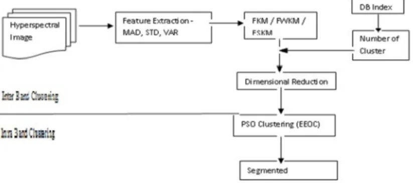
The band diminishing process could be carried out by one of these clustering methods, used to pick out one band from each cluster. 103 bands of the HSI are diminished to below twenty bands i.e. one band is preferred according to foremost variance from each cluster. The segmentation is carried out on the reduced band by applying the particle swarm clustering method. Moreover for segmentation, the proposed algorithm Enhanced Estimation Of Centroid (EEOC) is examined. It is the modification of general PSC by computing the particle that has updated their positions and reinstated the distance matrix only once per iteration. The flowchart of the proposed method (Fig. 1) is delineated.

Dataset description

Pavia Center scene was acquired by the ROSIS sensor during a flight campaign over Pavia, Northern Italy [2]. Originally, the number of spectral bands is 115 with 1096 x 1096 pixels. Some bands have removed due to noise. Finally, remaining 102 spectral bands are considered. The geometric resolution is 1.3 meters.

Fig. 1. Flow for fast K-Means technique for hyperspectral image segmentation by multiband reduction

4.1. Band reduction using FKM

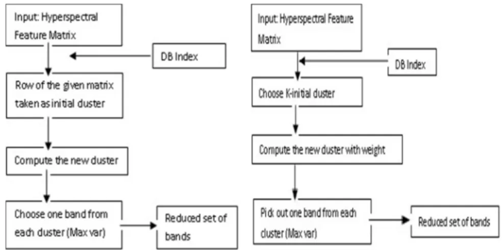
The FKM algorithm has used to diminish the hyperspectral band into below 20 as it is demonstrated in Fig. 2. The working principle of this approach is as follows.

Construct the hyperspectral feature matrix and the number of clusters (determined from DB index). A number of rows in the given matrix are taken as an initial cluster.

Compute the new cluster as like of K-Means and choose one band from each cluster which has maximum variance. More than 100 bands of the hyperspectral bands are reduced to below 20 bands, i.e. one band is selected according to the maximum variance from each cluster. Finally, the reduced set of bands has obtained.

4.2. Band reduction using FWKM

In FWKM, the hyperspectral band has reduced below 20 as it depicted in Fig. 3.

Construct the hyperspectral feature matrix and get the number of clusters (determine from DB index). Choose the K initial cluster centers and then, the new cluster is computed based on weight, i.e. more than 100 bands of the hyperspectral bands are reduced below 20 by pick out band as it was for previous method. Hence, the reduced set of bands has obtained.

4.3. Band reduction using FCSKM

In FCSKM, the hyperspectral feature band has reduced below 20 as it is shown in Fig. 4. Construct the hyperspectral feature matrix and get the number of clusters

(determined from DB index). Select the centroid randomly. Select the next cluster with the probability function D² weighting. If the number of cluster is equal to assign, then precede the next step, i.e. find the new cluster. Otherwise, repeat the same process. One band is picked out according to the maximum variance from each cluster as like of previous method. Finally, the reduced set of bands has obtained.

In this work, the lightweight clustering algorithm entitled as EEOC [4], [9] has examined. This algorithm is the modification of PSC. The modification has done on two levels. The Distance Matrix (DM) and best positions are updated after all particle positions are updated, i.e. the DM is restored only once per iteration.

Fig. 2. Band reduction using FKM Fig. 3. Band reduction using FWKM

Fig. 4. Band reduction using FCSKM

5. Experimental results

The fulfillment of EEOC algorithm is analyzed and experimented with various cluster methods such as FKM, FWKM, and FCSKM. It is applied in HSI - Pavia Center.

The results are generally compared with maximum iteration of 100. This work is executed in MATLAB v 10.

5.1. DB index graph

Fig. 5a depicts DB index graph. In X-axis, number of clusters (i.e. the value is incremented by 1 pixel) and in Y-axis, DB value (i.e. the value is increment by 0.05 pixel) is determined. In Pavia Center the DB-value is least at 19^th cluster. So, the DB index of this scene is considering as 19.

5.2. Output

Fig. 5a, portray the segmentation result for HSI Pavia Center is examined in FKM based on PSC (EEOC). Fig. 5b and Fig. 5c depict the segmentation result for this scene using FWKM and FCSKM.

5.3. Result analysis

The results are analyst in different scenario. First step is, analyzing the performance based on pixels; next analyzing is taken through as time complexity and fitness value.

a) b) c) d)

Fig. 5. Result for Pavia Center a) FKM + PSC (EEOC); b) FWKM + PSC (EEOC);

c) FCSKM + PSC (EEOC); d) DB index graph for Pavia Center scene Performance based on pixels

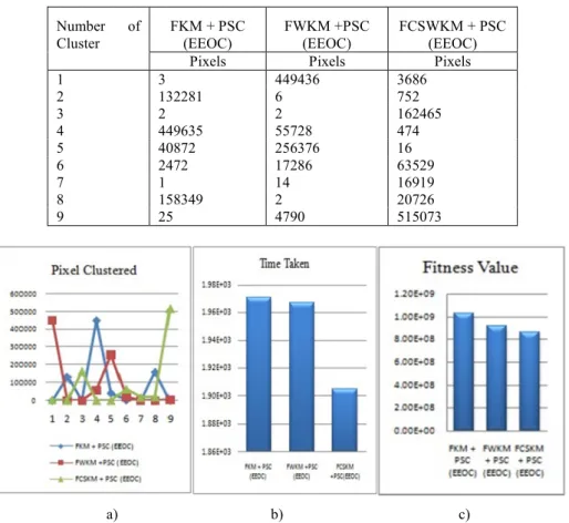
As per the reference to the ground truth image, the Pavia Center scene has segmented with nine clusters. The size of this scene is 1096 x 715 x 102. These 102 bands are reduced into 19 bands as per the Davies-Bouldin index and finally this 1096 x 715 pixels are clustered into nine, as 783640 pixels are grouped into these

clusters. The numbers of pixels are clustered as a result is portrayed in above Table I.

Fig. 6a depicts this result in chart form, Fig 6b depicts the time taken to execute for above-said approaches, and Fig 6c portrays the fitness value of these approaches.

Table I

Pixels clustered based on PSC (EEOC) with FKM Number of

Cluster

FKM + PSC (EEOC)

FWKM +PSC (EEOC)

FCSWKM + PSC (EEOC)

Pixels Pixels Pixels

1 3 449436 3686

2 132281 6 752

3 2 2 162465

4 449635 55728 474

5 40872 256376 16

6 2472 17286 63529

7 1 14 16919

8 158349 2 20726

9 25 4790 515073

a) b) c)

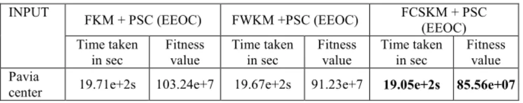
Fig. 6. a) Pixel Clustered chart, b) Time taken to execute chart, c) Fitness value chart The following Table II illustrates the time taken and fitness value for the above-said methods on the Pavia center HSI.

From Table II, FCSKM+PSC (EEOC) take minimum time for execution. The other two methods show close results to this method. Owing to this work particle swarm clustering method is used; the fitness value is one of the parameters to measure the accuracy. The least fitness value indicates the optimum results. Moreover Table II depicts the fitness value of EEOC worked with various Fast K-Means clustering methods. For Pavia Center, EEOC working with FCSKM gives the least fitness value. i.e. optimum.

Other methods yield a close result to FCSKM.

Table II

Elapsed time in seconds and fitness value INPUT

FKM + PSC (EEOC) FWKM +PSC (EEOC) FCSKM + PSC (EEOC) Time taken

in sec

Fitness value

Time taken in sec

Fitness value

Time taken in sec

Fitness value Pavia

center 19.71e+2s 103.24e+7 19.67e+2s 91.23e+7 19.05e+2s 85.56e+07

6. Conclusion

This paper addresses about segmentation of hyperspectral remote-sensing satellite scene. The unsupervised clustering methods, for instance, FKM, FWKM, and FCSKM are inspected with PSC (EEOC). DB index used to determine the number of cluster. The above-said clustering strategies are applied on hyperspectral feature matrix, and this matrix is clustered and a band, which has foremost variance from each cluster, is picked out. In inter clustering part the band sizes are reduced into below twenty. In intra-band clustering part, segmentation is carried out on this reduced band by PSC-EEOC.

Furthermore, the result generated by this approaches is analyzed in different scenario.

To be crisp, FCSKM with PSC-EEOC produce the best result in terms of time complexity and fitness values. Despite taking minimum time, the above introduced methods are lead the over segmentation.

References

[1] Plaza A., Benediktsson J. A., Boardman J., Brazile J., Bruzzone L., Camps-Valls G., Chanussot J., Fauvel M., Gamba P., Gualtieri A., Marconcini M., Tilton J. C., Trianni G.

Recent advances in techniques for hyperspectral image processing, Remote Sensing of Environment, Vol. 113, No. 1, 2009, pp. S110‒S122.

[2] Kumar V. S., Naganathan E. R. A survey of hyperspectral image segmentation techniques for multiband reduction, Australian Journal of Basic and Applied Sciences, Vol. 9, No. 7, 2015, pp. 446‒451.

[3] Jain A. K., Murty M. N., Flynn P. J. Data clustering: a review, Association of Computing Machinery, Computing Survey, Vol. 31, No. 3, 1999, pp. 264‒323.

[4] Veligandan S. K., Rengasari N. Hyperspectral image segmentation based on enhanced estimation of centroid with Fast K-Means, The International Arab Journal of Information Technology, Vol. 15, No 5, 2018, pp. 901‒911.

[5] Zhang B. Generalized K-harmonic means- boosting in unsupervised learning, HP Labs Technical Report, HPL‒000‒137.

[6] Kumar V. S., Naganathan E. R. Segmentation of hyperspectral image using JSEG based on unsupervised clustering algorithms, ICTACT Journal on Image and Video Processing, Vol. 6, No. 2, 2015, pp. 1152–1158.

[7] Arthur D., Vassilvitskii S. K-means++: The advantages of careful seeding, SODA '07 Proceedings of the Eighteenth Annual ACM-SIAM Symposium on Discrete Algorithms, New Orleans, Louisiana, US, 7-9 January 2007, pp. 1027‒1035.

[8] Saatchi S., Hung C. C. Swarm intelligence and image segmentation, in: Swarm Intelligence: Focus on Ant and Particle Swarm Optimization, Ed. by Felix T. S. Chan, Manoj Kumar Tiwari, Itech Education and Publishing, Vienna, Austria, 2007, pp. 163‒178.

[9] Kumar S. V, Prakasam A. S., Rengasari N. E., Kavitha M. Multiband image segmentation by using enhanced estimation of centroid (EEOC), Information, Journal in Japan, Vol. 17, No. 6, 2014, pp. 1965‒1980.

[10] Ray S., Turi R. H. Determination of number of cluster in K-Means clustering and application in color image segmentation, Proceeding of the 4th International Conference on Advances in Pattern Recognition and Digital Techniques, Calcutta, India, 28-31 December 1999, pp. 137‒143.

[11] Jun L., Bloucas-Dias J. M., Plaza A. Spectral-spatial hyperspectral image segmentation using subspace multinomial logistic regression and Markov random field, IEEE Transaction on Geosciences and Remote Sensing, Vol. 50, No. 3, 2012, pp. 809‒823.

[12] Plaza A., Valencia D., Plaza J., Martinez P. Commodity cluster-based parallel processing of hyperspectral imagery, Journal of Parallel and Distributed Computing, Vol. 66, No. 3, 2006, pp. 345‒358.

[13] Tamas S., Ercsey Zs., Varady G. Histogram based segmentation of shadowed leaf images, Pollack Periodica, Vol. 13, No. 1, 2018, pp. 21‒32.

[14] Tarabalka Y., Benediktsson J. A., Chanussot J. Spectral-spatial classification of hyperspectral imagery based on partitional clustering techniques, IEEE Transactions on Geoscience and Remote Sensing, Vol. 47, No. 8, 2009, pp. 2973‒2987.

[15] Szabo A., de Castro L. N. A constructive data classification version of the particle swarm optimization algorithm, Mathematical Problems in Engineering, Vol. 2013, pp. 1‒13.

[16] Mohsen F., Hadloud M., Mostafa K., Amin K. A new image segmentation method based on particle swarm optimization, The International Arab Journal of Information Technology, Vol. 9, No. 5, 2012, pp. 487‒493.

[17] Kumar V. S., Naganathan E. R. Hyperspectral image segmentation based on particle swarm optimization with classical clustering methods, Advances in Natural and Applied Sciences, Vol. 9, No. 12, 2015, pp. 45‒53.

[18] Cserhalmi D., Nagy J., Neidert D, Kristof D. The reconstruction of vegetation change in Nyires-to mire (in Hungary): An image segmentation study, Acta Botanica Hungarica, Vol. 52, No. 1-2, 2010, pp. 89‒102.

[19] Tepavcevic B., Sijakov M., Sidanin P. Gis technologies in urban planning and education, Pollack Periodica, Vol. 7, Suppl. 1, 2012, pp. 185‒191.