A fuzzy clustering method for periodic data, applied for processing turbomachinery beamforming maps

A fuzzy clustering method for periodic data, applied for processing turbomachinery beamforming maps

Bence T´oth^a,∗, J´anos Vad^a

aDepartment of Fluid Mechanics, Faculty of Mechanical Engineering, Budapest University of Technology and Economics. Bertalan Lajos u. 4-6, H-1111 Budapest, Hungary

Abstract

In the present paper, the fuzzy c-means method is extended, and an algorithm is proposed for fuzzy clustering of data lying in a feature space of arbitrary dimensions, with one of them being periodic. To aid in determining the op- timal number of clusters, the Xie-Beni validity index is extended, to account for the periodicity. Furthermore, the relative weights of the dimensions in the calculation of distances are investigated. The method is incorporated into a procedure for processing turbomachinery beamforming maps. Thus, an objec- tive, robust way of identifying the sound sources being present in such machines is obtained. These properties are ensured by selecting the required parameters through parameter studies. Presented through a case study, the method is used to determine the most significant sound source mechanisms in an axial fan.

Keywords: axial flow fan, beamforming, fuzzy clustering, periodicity 2010 MSC: 00-01, 99-00

Nomenclature

Latin letters

∗Corresponding author

Email address: tothbence@ara.bme.hu(J´anos Vad)

a element of the weighting matrix A weighting matrix

B number of fan blades c number of fuzzy clusters d distance metric

D number of data set dimensions f frequency

i index of data points I identity matrix j index of clusters

J clustering objective function k period tracking variable l running index

m fuzzifier

N number of all data points to be clustered p dimensionless amplitude

p periodic offset vector P period

R dimensionless radius s iteration step w membership value x generic vector y generic vector Greek letters

β angular position of base source γ arbitrary periodic quantity exit criterion residual µ cluster centre

σ cluster amplitude ξ data point for clustering

5

Superscripts and subscripts

A weighted using matrixA min minimum

max maximum

P periodic distance measure T transpose

Abbreviations

AMP & ADC Amplifier and analogue-to-digital converter FCM Fuzzy c-means clustering

FCM4DD Fuzzy c-means clustering for directional data

LE Leading edge

PAM Phased array microphone

PC Personal computer

ROSI Rotating source identifier SPL Sound pressure level

TE Trailing edge

XB Xie-Beni index

Others

10

ˆ normalised to the 0 . . . 1 range

1. Introduction

The noise emitted by turbomachinery is a serious issue. To reduce it, the noise generation mechanisms have to be identified, understood, and controlled.

Acoustic beamforming can effectively be used for indicating the areas where

15

the strongest sources of noise are present [1, 2, 3]. Some approaches can han- dle rotating systems [4, 5, 6, 7], enabling the investigation of turbomachinery.

Beamforming measurements are often carried out on aero-engines due to noise emission limits becoming more strict. In the recent years, investigation of low- speed axial fans has begun, as they operate in larger numbers and closer to

20

people [8, 9, 10]. Combined with empirical analysis and numerical simulations, as done in [11, 12, 13, 14, 15], the information regarding source locations can aid in understanding noise generation mechanisms. Then an iterative redesign

process can be started, within which, by modifying the blade geometry, the noise emission can be reduced.

25

The results of beamforming are usually presented in the form of contour maps over the target, in the present case, over the rotor. These are called beamforming maps. These maps are usually interpreted visually. This process however includes subjective elements. Furthermore, such maps are usually gen- erated for several frequency bands, in which case, drawing conclusions based on

30

them is even more difficult.

The situation is further complicated by the presence of point spread func- tions in the maps. Due to these, a point-like source appears with a spatial ex- tension, and close-by sources become difficult to separate. Furthermore, peaks may appear at locations where in reality no sources are present. These effects

35

are usually treated using deconvolution methods, such as CLEAN-SC [16] or DAMAS [17], however, in some cases, these algorithms may not be applicable.

Yet, the aforementioned problems have to be tackled in some way.

To do that, a novel algorithmic processing method was proposed in [18, 19]. It aimed at the identification of noise generation mechanisms through a

40

data reduction and clustering procedure. This was illustrated in a case study, and found adequate, however, still contained a subjective choice due to the periodicity of the blading.

The main contribution of the present paper is to introduce a method for fuzzy clustering, applicable when one of the dimensions of the data set has

45

periodic attributes. This is applied for the analysis of turbomachinery beamform maps as part of the aforementioned algorithm [19], aimed at objective and reproducible identification of noise source mechanisms. The extended algorithm is applied onto the beamform maps of an axial fan, to identify the dominant noise generating mechanisms.

50

In the present application, the novel procedure ensures that clustering takes the periodicity of the blade passages into account, even if only one blade passage is used for data analysis. However, it may be applied for any kind of data, where a periodic dimension is present.

The structure of the paper is as follows. First, the complete method for

55

source identification is described. Second, the original fuzzy clustering algo- rithm is presented, the meaning and the difficulty of clustering in the presence of periodic dimensions is explained, and the modified clustering algorithm is introduced. Third, details about the case study are given. Fourth, the results of applying the new algorithm onto the beamforming data are presented and

60

compared to those of the previous method. Finally, the conclusions of the work are summarised.

2. Noise source identification method

To investigate and analyse turbomachinery noise, a novel algorithmic ap- proach was proposed in [18, 19]. It aimed at identifying broadband noise gen-

65

eration mechanisms in an axial fan, in an objective manner. The method was designed to decrease the effects of both measurement noise and side lobes, with- out deconvolution. The reason for omitting deconvolution methods was that a microphone array with generic microphone placement was used in the measure- ments, and thus the beamform maps were created using the Rotating Source

70

Identifier (ROSI) [4]. As this method does not provide a cross spectral ma- trix that would describe the source effects, the widely applied deconvolution methods were not applicable.

The approach was illustrated on beamforming data taken from the tip radius of an axial fan. The significant features of the beamforming maps were repre-

75

sented as points in the circumferential angle (β) – frequency (f) plane [β, f], thus the identifiedbase sources were described by their location around the ro- tor, and by frequency of their emitted sound. Those data points that are likely signatures of the same noise generation mechanism, were grouped through a clustering procedure. The identified clusters were then assigned to known noise

80

generation mechanisms based on previous literature.

In the previous paper [19], the algorithm was applied to one blade passage only, as the periodicity of the noise sources was assumed and enforced in a filter-

ing process. This was done to reduce sidelobe, large-scale turbulence ingestion, inflow irregularity, local geometric irregularity, and measurement uncertainty

85

effects.

The steps of the method were the following.

1. For each investigated frequency band, a circumferential source strength distribution was extracted from the beamforming maps around the rotor at a selected radius.

90

2. The distributions obtained in the previous step were expanded into spatial Fourier series.

3. From each Fourier series, only those modes were considered, whose cir- cumferential wave number conformed to the periodicity of the blading.

This means that the number of periods of the harmonic wave in one blade

95

passage is a positive integer. Through this step, noise sources not directly related to the rotor are filtered out. This way, the effects of those peaks in the maps are reduced, that do not have spatial periodicity: e.g. side lobes, large-scale turbulence ingestion noise, and other artefacts.

4. Important components were selected using a significance criterion based on

100

theirpmodal amplitudes. The significance limit was the largest amplitude in the spectrum found at a circular wave number that does not agree with the periodicity of the blades, i.e. the largest amplitude of those modes, that have non-integer periods inside one blade passage. This reduces the number of data points, and further reduces measurement uncertainties.

105

5. Each significant mode was considered as abase source. A base source is a point in the circumferential angle – frequency plane [β, f].

6. Clusters were created from the base sources, based on the distances be- tween them, using a fuzzy clustering procedure allowing for overlapping.

7. The source mechanisms corresponding to the clusters were identified.

110

Application details and further explanation for the individual steps can be found in [19].

As mentioned above, only those sources are considered important, that con- form to the periodicity of the blade passages. This periodicity was enforced through the Fourier analysis and filtering. Therefore, choosing one blade pas-

115

sage for analysis and clustering was sufficient, as they all contain the same base sources. However, one had to choose the limits of theanalysis window, i.e. the part of the [β, f] plane in which clusters are sought for. Physical arguments were followed in thef direction, but in the angularβ direction, due to the repeating blade passages, no objective decision could be made as to where a blade passage

120

periodic noise pattern begins. After a visual inspection, the beginning of the analysis window, β = 0 was assigned to the blade trailing edge. This choice however could have significant effects on the results of clustering, which should be avoided.

A further problem regards the calculation of distances required by the clus-

125

tering method. Even though the quantities are normalised before clustering, the dimensions ofβandf are different. Therefore no physical reasoning can be given as to how to calculate the distance between two points in this plane.

To overcome these problems, a modified fuzzy clustering method is proposed, being able to take periodicity in the data set into account. This way, the begin-

130

ning of the analysis window,β= 0, can be assigned arbitrarily, as the resulting clusters will not depend on that. Besides the present case, the method will suit any application, where one of the dimensions is periodic. Furthermore, the ef- fects of different dimensions in the distance calculations will be investigated in a case study. In this paper, the method is applied not only onto the tip radius,

135

but at other radii in the rotor annulus area, as well.

3. Clustering

Clustering is a process of assigning data points to groups, based on their similar attributes. The general task is the following. Knowing theξ_i, i= 1. . . N data points, lying in the so-calledfeature space ofDdimensions, determine the

140

prescribed c number of cluster centres µ_j, j = 1. . . c, such that an objective

function, the error regarding the replacement of the data points with the cluster centres, is minimised. For the sake of simplicity, the data points are assumed to be normalised onto the range 0, ..., 1 in each dimension.

This section summarizes the original fuzzy clustering method, the properties

145

of periodic data, and introduces the modified clustering algorithm that accounts for a periodic dimension.

3.1. Fuzzy c-means clustering

Several clustering methods have been proposed. Possibly the simplest al- gorithm is the k-means method [20]. In this case, all data points are assigned

150

to the closest cluster, while the cluster centres are determined as the weighted average of the assigned data points. Since one data point belongs to one cluster only, this clustering method is termedcrisp.

Fuzzy c-means clustering (FCM) [21] is a method similar to k-means, but in this case, the clusters are considered fuzzy. This means that one data point

155

may belong to more clusters, and therefore the clusters may overlap.

As noted before, clusters are identified by minimising an objective function.

In FCM, this is the sum of the weighted squared distances between the cluster centres and the data points. The objective function is shown in Eq. (1). The aim is to find cluster centresµ_j, j = 1. . . c that minimise this expression.

J=

N

X

i=1 c

X

j=1

w^m_i,jd² ξ_i,µ_j

(1) In Eq. (1), ddenotes the distance measure between any two points in the feature space. This will be investigated in detail later. wi,j ∈ [0,1] values are the so-calledmembership values, quantifying how well a data point ξ_i fits into thej-th cluster. The sum of these for one data point over thecclusters is unity, as shown in Eq. (2). The application of membership values gives the possibility for overlapping clusters.

c

X

j=1

wi,j= 1 ∀i (2)

The parameterm >1 is thefuzzifier that controls the level of separation of the clusters. Its behaviour will be discussed later.

The objective functionJcan be interpreted as follows, based on [21]. d² ξ_i,µ_j is the squared distance between data pointξ_i and cluster centreµ_j. The term

160

wi,jd² ξ_i,µ_j

is the error – weighted by the membership raised to a certain power – that arises when µ_j is taken to represent ξ_i. The two summations mean that this error regarding one data point and one cluster centre has to be added up considering each data point – cluster centre combination. Thus a total error is obtained. Minimising this total error means finding cluster centres

165

representing the data points at the best. This is achieved by the FCM algorithm by iteratively calculating the cluster centres and the membership values.

The location of each cluster centre is determined by averaging the data points, weighted by their membership values regarding that cluster. This is shown in Eq. (3).

170

µ_j = PN

i=1w^m_i,jξ_i PN

i=1w_i,j^m (3)

For the calculation of thewi,j membership values, Eq. (4) is used.

wi,j=

c

X

l=1

d(ξ_i,µ_j) d(ξ_i,µ_l)

_m−1² !⁻¹

(4) The role of wi,j can better be understood by rewriting Eq. (4) in another form, shown in Eq. (5).

wi,j=

1 d²(ξ_i,µ_j)

_m¹₋₁

Pc l=1

1 d²(ξ_i,µ_l)

_m−1¹ (5) By looking at Eq. (5), and considering the reciprocal of the squared dis- tances, _d¹2 as a measure of closeness, one can see howwi,jbehaves. This formula

175

assigns a large membership value to a cluster – data point pair if they are close to each other (their “closeness” is large), but a small one, if they are remote. It also ensures that the condition in Eq. (2) is fulfilled, since the numerator is a

normalisation by the sum of all membership values regarding the chosen data point.

180

How steeply thewi,jmembership values changes with the distance is defined by the fuzzifier. Asm→1, the exponents in Eq. (5) grow, therefore the cluster centre being closest to the data point will dominate the denominator, thus that membership value will be close to unity, and necessarily, the other ones will be small. Therefore the overlap between the clusters decreases, and they become

185

crisper. On the other hand, asm→ ∞, the exponents tend to zero, therefore the effects of different distances vanish, and all the terms in the denominator will be similar in magnitude. Thus all wi,j →1/c, meaning that the clusters spread out, the overlap grows, and the ability to differentiate between clusters disappears [21].

190

In FCM, the aforementioned expressions are used until the results converge to finalwi,j and µ_j values. Details on convergence can be found in [21]. The algorithm is the following.

1. wi,jvalues are initialised randomly, but fulfilling the constraint in Eq. (2) 2. Cluster centres are calculated using Eq. (3)

195

3. Membership values are updated using Eq. (4)

4. The process is continued from Step 2 using the new values until conver- gence is reached.

Convergence is checked by comparing the matrices composed of the wi,j

values obtained in the present and the previous step. If the norm of the difference

200

of these matrices is smaller than a pre-specified limit, the algorithm terminates.

This method has proven its capability to identify clusters in several cases, some relevant ones being the following. FCM was applied for microphone array measurements in reverberant environments [22, 23], to aid in source localisa- tion. The vortex field behind an oscillating cylinder was analysed in [24], while

205

turbulent flow patterns were investigated in [25].

Two effects require further analysis regarding the application of FCM in the present case. First, the relative importance of frequency and angular data in

identifying clusters should be investigated. This is done in the next section in the form of the distance metric. Second is the periodicity of the fan blading, causing

210

the noise patterns to be periodic. Due to this, it is sufficient to investigate the noise pattern in one blade passage only. To do clustering in one blade passage, one has to assign the passage a beginningβ= 0 angular position, which can not be done in an objective way. Furthermore, this choice may change the result of clustering if periodicity is not taken into account. To avoid the influence of

215

this arbitrary choice, the FCM clustering algorithm was extended to handle a periodic dimension. This way the result of clustering will be the same for a data set, regardless of where β = 0 was chosen. This problem and its solution will further be discussed in later subsections.

3.2. Distance weights

220

FCM relies on the ddistance between any two points in the feature space, here denoted byxandy. This may be the Euclidean norm in the simplest case, e.g. d(x,y) =||x−y|| =

q

(x−y)^T (x−y). However, the dimensions of the feature space before non-dimensionalisation may have different physical units, or have significantly different ranges. In this cases, one may have to alter the

225

way the distances are calculated even after the data was made dimensionless, to modify the importances of the different dimensions in clustering. This is achieved by using weights in the calculation of distances. These weights are incorporated into the matrixA.

The weighting is introduced through the following scalar product definition:

hx,yi = x^TA y [21]. With this, the distance metric induced by matrix A is that shown in Eq. (6).

dA(x,y) =||x−y||A= q

(x−y)^TA(x−y) (6) In the simplest approach, A = I, the identity matrix. In this case, the

230

Euclidean norm is obtained. Some other approaches are described in [21]. In the present case, a diagonal matrix is applied, shown in Eq. (7), with a1 = 1 as the weight for the first dimension, and adjustableak, k= 2. . . D values for

the other dimensions. In this case, theak parameter controls the weight of the k-th dimension compared to the first one.

235

A= diag(1, a2, a3, . . . aD) (7) This is a flexible approach, allowing to set how much influence one dimen- sion has in clustering. However, there are no generally valid guidelines about the choice of theakweights. This problem is especially relevant, when the data consists of quantities that are not physically comparable. To this end, a pa- rameter sensitivity study is proposed to determine theak values that provide

240

an acceptable clustering result, being in agreement with the properties of the clustering validity method, detailed later.

3.3. Periodicity

When periodic and non-periodic dimensions are both present, the data set is termedhybrid, following ref. [26]. The present subset, with exactly one periodic

245

and one non-periodic dimension, is termed cylindrical [27]. FCM has been widely used for clustering different types of data, however, it cannot directly be applied onto data with periodic attributes, such as the noise pattern according to the periodicity of the blades in the present case.

To apply FCM onto cylindrical data, one has to consider only one period

250

of the infinitely long periodic dimension. This is termed theanalysis window.

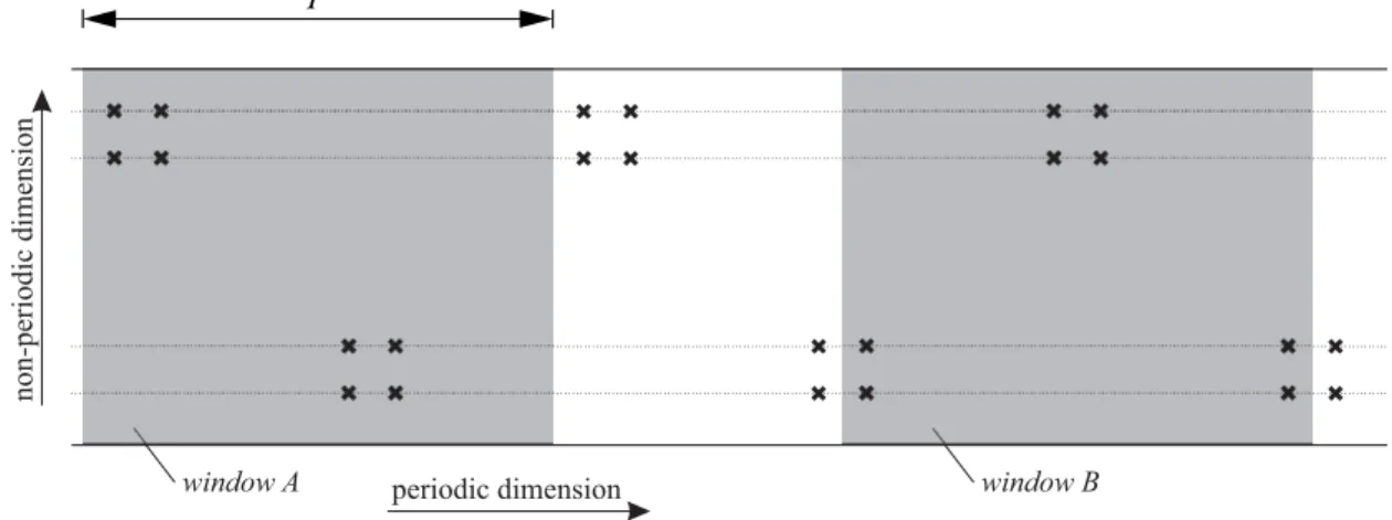
Where this analysis window begins in the periodic dimension, is a subjective choice, that can seriously influence the result of clustering. This effect is shown on an illustrative hybrid data set in Fig. 1. There, a hybrid data set is shown, with the horizontal axis being periodic with a repeating data pattern, while the

255

vertical dimension is non-periodic. The crosses indicate the data points. In order to do clustering, one has to define the position of the analysis window, i.e.

choose the origin of theβ coordinate. This cannot be done based on a physical argument, due to the periodic nature of the dimension. However, this choice may determine the result of partition.

260

Windows A and B show two possible choices forβ= 0 and thus the location of the analysis window. Note however, that just by visual observation, one can conclude that in window A, two clusters exist, while window B contains three.

This illustrates the possible problems of clustering periodic data.

One may decide that window A is beneficial, as it does not cut a cluster into

265

two pieces. This would however be a subjective choice, which may not even be applicable when the number of data points N is high. Furthermore, this approach disregards the periodic nature of the data set, leading to incorrect membership values. To avoid this, the clustering method is to be modified to handle cylindrical data. The task is then to cluster data sets lying in a

270

periodic/hybrid domain, in a way that the resulting clusters are invariant to the choice of the analysis window. To reach this, in case of a purely periodic or hybrid data set, distances required for clustering have to be calculated by taking the periodicity into account.

non-periodic dimension

periodic dimension P

window A window B

Figure 1: Illustration of the effects of arbitrarily assigned analysis windows in case of hybrid data. The horizontal axis is a periodic dimension, while the vertical is non-periodic. Shaded areas indicate two possible analysis windows. If periodicity is not considered, two clusters are observed in window A, while in B, three.

An approach for clustering periodic data using the k-means algorithm is

275

treated in [26]. Besides some other methods, the authors propose the following

metric, defined along a periodic dimensionγ with periodP, shown in Eq. (8).

dP(γ1, γ2) = min{|γ1−γ2|, P − |γ1−γ2|} (8) Furthermore, they discuss the treatment of hybrid data, as well. The method is suitable for k-means clustering, however, it was not extended for fuzzy clus- tering.

280

For FCM, the fuzzy c-means algorithm for directional data (FCM4DD) was proposed in [28]. The method was compared against other methods, reported in [29] and [30], and performed favourably, giving better results, while requiring less computational effort. However, in this algorithm, only periodic dimensions can be taken into account, e.g. FCM4DD is not suitable for hybrid data.

285

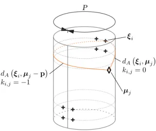
Thus, solutions exist for non-fuzzy clustering of hybrid data, and fuzzy clus- tering of purely periodic data. The novelty of this paper is an approach to create fuzzy clusters in hybrid data sets. The idea behind the method is illustrated by Fig. 2. It shows the same points as in Fig. 1, however, now the data set is wrapped around a cylinder. If the surface of the cylinder is considered for

290

calculating distances and for clustering, periodicity can successfully be taken into account. While Fig. 2 illustrates a two-dimensional hybrid case, the same idea can be applied for more dimensions, as well.

To implement this idea, the distance norm is modified similarly to Eq. (8).

This way, distance can successfully be calculated in a periodic/hybrid data set,

295

and the results are not dependent upon the arbitrary selection of the analysis window.

3.4. Method for fuzzy clustering of hybrid data

The proposed method is able to create fuzzy clusters similarly to FCM, with a hybrid data set, whereexactly one dimension is periodic. In the following,

300

without loss of generality, the first dimension is considered as being periodic, with periodP.

All dimensions are to be normalised to the range 0 . . . 1. AD-dimensional periodic offset vector is introduced, shown in Eq. (9), with the period being

P

Figure 2: Interpretation of the periodic distance norm. The analysis window is wrapped onto a cylinder.♦: cluster centre, +: data point. The two possible lines connecting cluster centre µ_jandξ_iare shown.

unity after normalisation. Thereforepis the unit vector in the periodic dimen-

305

sion, regardless ofD.

p= [1,0, . . .0]^T (9)

The periodic, weighted distance metric dA,P is to be applied, shown in Eq.

(10). It is based on Eq. (6), but was extended for a hybrid case usingp. This includes the diagonal weighting matrix shown in Eq. (7).

dA,P = min{dA(ξ_i,µ_j−p), dA(ξ_i,µ_j)} (10) This means that every time the distance between data point ξ_i and centre µ_j is required, it has to be considered that a counterpart of µ_j exists in the previous data window as well. The position of this counterpart isµ_j−p. For the algorithm, the smallest of the two distances are to be considered. This is

310

analogous to finding the distance on the cylinder shown in Fig. 2, where two points on the surface can be connected from two directions, but the length of the shorter path is defined as their distance.

This distance norm however will often impede convergence. The reason is that when the new cluster centres are calculated, in Eq. (3), the averaging

315

of the data points will again place the µ_j somewhere in between them. To reach convergence even in this case, it is necessary to track, whether the data pointξ_iis closer to centreµ_jfrom the current analysis window, or to its periodic counterpartµ_j−pin the previous analysis frame. In the analogy of the cylinder, this means considering, in which direction were the two points closer to each

320

other. Keeping track of this is done by a new variableki,j ∈ {−1,0}. Its possible values are shown in Eq. (11).

ki,j =







−1 if dA(ξ_i,µ_j−p)< dA(ξ_i,µ_j) 0 otherwise

(11) ki,jis used to indicate if pointξ_iis closer toµ_jin the present analysis window (ki,j = 0), or to its periodic counterpart in the previous window (ki,j =−1).

The k values are shown in Fig. 2 together with the two paths. ki,j = −1

325

belongs to the case, when the line connectingξ_i andµ_j crosses the generatrix corresponding to the 0 value of the periodic dimension. By using ki,j, the cluster centres can successfully be calculated following Eq. (12). This way, the algorithm takes into account, which periodic counterpart of the data point is closer to the centre, and will use that for the calculation of the new centre

330

location.

µ_j= PN

i=1w^m_i,j(ξ_i+ki,jp) PN

i=1w_i,j^m (12)

When these are obtained, the membership values can be updated. This is reached by using Eq. (4), but by taking the periodic weighted distance norm dA,P into account, as shown in Eq. (13).

wi,j=

c

X

k=1

dA,P(ξ_i,µ_j) dA,P(ξ_i,µ_k)

_m−1² !⁻¹

(13) The algorithm is the following.

335

1. Set c, m, A, p, , ki,j = 0, and initial wi,j values. Then repeat the following steps fors= 1,2. . . smax

2. Compute centres µ^(s)_j , j = 1,2. . . c using Eq. (12). If the periodic coordinate ofµ_j leaves the domain [0,1), reintroduce it to the other side by taking its fractional part.

340

3. Computek^(s+1)_i,j using Eq. (11).

4. Compute membership valuesw^(s+1)_i,j using Eq. (13).

5. Compare the matrices constructed from the wi,j membership values at steps s and s+ 1. If the norm of their difference is less than , exit.

Otherwise, incrementsand return to step 2.

345

3.5. Xie-Beni index

A limitation of FCM is that the number of clusters c is to be known in advance [31]. This information is, however, generally not available. Therefore the suggested procedure is to employ a parameter sensitivity study by varying c. During that, a measure of clustering goodness is to be investigated. These

350

measures are called validity indices. Many kinds exist, some of them being summarised in [31]. In the original method in [19], the Xie-Beni (XB) index [32]

is used, as it is easy to compute, yet able to quantify the two most important aspects of good clustering:

• compact clusters are sought for,

355

• being well-separated from each other.

The XB index is defined in Eq. (14).

XB = PN

i=1

Pc

j=1w^m_i,jd²(ξ_i,µ_j) N min

j6=l d²(µ_j,µ_l) (14)

In Eq. (14), the numerator is in relation to the error introduced by replacing the data points with the cluster centres, therefore the lower this value, the more compact the cluster. The denominator contains the distance of the two clusters

360

lying closest to each other, being a measure of cluster separation. In this case,

the higher its value, the better the clustering. Based on these, the minimum XB value indicates the optimal clustering, and the optimal choice ofc.

The periodicity in the data set has to be accounted for in the calculation of XB, as well. This is straightforward, as only the distance measures have to

365

be changed to the new, weighted and periodic ones. The periodic XB index is shown in Eq. (15).

XBP = PN

i=1

Pc

j=1w_i,j^md²_A,P(ξ_i,µ_j) N min

j6=l d²_A,P(µ_j,µ_l) (15)

3.6. Summary of the proposed clustering method

The outline of the method for fuzzy clustering of cylindrical data is the fol- lowing. First, an arbitrary analysis window is to be chosen, and the normalised

370

ξ_i values are to be calculated. Then hybrid fuzzy clustering is to be applied, using the algorithm above. This is to be repeated with all combinations of the investigatedc, m and ak values. Following that, parameter studies are to be carried out to determine the optimal settings for these variables. The optimal one, based on the XBP index and physical considerations, is to be chosen and

375

accepted. Finally, clustering results can be used and interpreted corresponding to the selected settings.

4. Case study

The present investigation concerns the same axial fan and the same measure- ment data as in [19]. Relevant details of the measurement setup are as follows.

380

The investigated fan was an axial flow industrial cooling fan, in a free-inlet free- exhaust rotor-only configuration. It was mounted in a short duct with a short inlet cone. The tip diameter of the fan was 0.3 m, the hub-to-tip ratio was 0.35, and the number of blades was 5. The rotor speed was measured by means of an optical probe, and found to be 1430 revolutions per minute. The tip gap size

385

was 7 mm. The blades were manufactured from steel plates with a circular arc camber profile. The blade tip, the trailing, and the leading edges were rounded.

An OptiNav, Inc. Array 24 phased array microphone was used for measuring the noise. This unit has 24 omnidirectional electret microphones mounted flush against the array surface. They are arranged along logarithmic spiral arms.

390

The diameter of the circumscribed circle is 0.95 m [3]. The array was placed perpendicularly to the fan axis of revolution, while the distance between the array and the fan inlet plane was 1.83 tip diameters. This distance was chosen to improve the spatial resolution of the beamforming maps, while avoiding inflow disturbances. The latter was confirmed in [14] for the same configuration. The

395

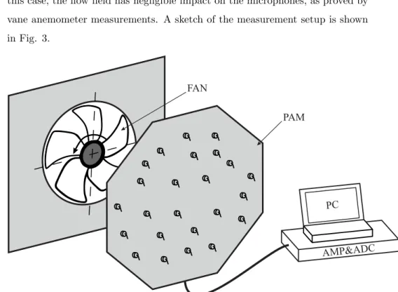
inlet velocity profile with and without the array was measured, and no significant difference was found. Measurements taken on the suction side are processed; in this case, the flow field has negligible impact on the microphones, as proved by vane anemometer measurements. A sketch of the measurement setup is shown in Fig. 3.

400

PC

AMP&ADC FAN

PAM

Figure 3: Sketch of the measurement setup. PAM: phased array microphone. AMP&ADC:

amplifier and analogue-to-digital converter. PC: personal computer. The microphone posi- tions are for illustrative purposes only; they do not correspond to those of the actual array.

The electric signals were amplified, digitised, and recorded by the accompa-

nying signal processing unit. A sampling frequency of 44.1 kHz was applied and data was acquired for 20 s, corresponding to more than 2000 blade passages.

The measurements were carried out in a laboratory with no special acoustical treatment. To remove the effects of rotation and create source maps in a sys-

405

tem rotating together with the rotor, the ROSI method was used [4], as the geometry of the array did not allow the application of frequency domain inter- polation methods, e.g. [33]. Frequency-domain information was obtained by cutting the data into blocks of 1024 overlapping by 50%, windowing them using a von Hann function, applying a fast Fourier transform on each block, then

410

averaging the spectra. Diagonal removal was applied to reduce the effects of uncorrelated noise between the microphones [4]. The narrow-band source maps were summed to create third-octave band maps centred on 2000, 2500, 3150, 4000, 5000, and 6300 Hz. Lower frequencies were omitted due to limitations in spatial resolution.

415

The sound pressure spectrum of the noise emitted by the fan, as measured by one microphone of the array, is shown in Fig. 4. It can be seen that in the investigated frequency range, the generated noise has broadband characteristics.

Therefore tonal noise was not investigated, and only broadband source mech- anisms were considered. Furthermore, this is why analysis with third-octave

420

band frequency resolution was considered appropriate.

The originally obtained beamform maps are shown in Fig. 5. Here one can see that the most significant noise sources are often in the vicinity of the rotor tip radius. However, the features are not completely periodic, which might be the result of some surface inhomogeneity, inflow effects, background noise,

425

measurement uncertainty, or side lobes from beamforming. These effects are however to be filtered out, as at this stage, the basic behaviour of the fan is to be investigated. The reason for applying the data reduction method is to remove these effects, to be able to concentrate on the remaining phenomena.

A further aim is to reduce these maps, that can only be inspected visually,

430

into a data set, that can easier be interpreted, in an algorithmic, reproducible manner. This is done by constructing the base sources, clustering them to find

f [Hz]

10² 10³ 10⁴

SPL[dB]

-40 -20 0 20 40 60

Figure 4: Noise sound pressure level spectra in dB [19]

those that are the result of the same mechanism, and then finding the relevant source mechanisms.

Possible broadband noise source mechanisms that may appear in low speed

435

axial fans in general are the following [19].

• Small scale turbulence ingestion noise. Noise originating from the turbu- lence of upstream flow, e.g. caused by a protection grid, impinging on the leading edge.

• Noise due to ingestion of large scale turbulence. This source is due to the

440

ingestion of large eddies, e.g. those shed by the housing, etc.

• Turbulent boundary layer noise. This noise originates from wall pressure fluctuations due to turbulence in the boundary layer.

• Separated flow noise. It is a result of the pronounced flow unsteadiness in case of flow separation.

445

• Profile vortex-shedding noise. This originates from the vortices being shed over the blade profile.

• Turbulent boundary layer – trailing edge interaction noise. This noise is the result of scattering turbulence at the trailing edge in case of an

Figure 5: Third-octave band beamforming maps [19] at mid-frequencies between a) 2 kHz and e) 6.3 kHz. The colour bar shows the beamform levels in dB, while the circle indicates the Rayleigh resolution limit at the mid-frequency of the third-octave band.

attached boundary layer.

450

• Tip leakage flow noise. This noise is generated by the highly turbulent tip leakage flow coming from the preceding blade.

• Double leakage flow noise. Similar to the previous noise, but the flow is coming from the second preceding blade.

• Blunt trailing edge vortex shedding noise. This noise source is the result

455

of vortices being shed at the finite thickness of the trailing edge.

Out of these, the noise sources identified using the clustering method will be presented in the Results section. The original beamform maps are treated in detail and compared to computational fluid dynamics studies in [13, 14, 15].

Since third-octave band beamforming maps were filtered and evaluated, the

460

base sources refer to the mid-frequencies of these bands. However, these repre- sent the whole frequency range between the lower and the upper limit frequen- cies of that third-octave band. Due to this, the normalisation procedure in Eq.

(16) was applied. Here (fmin) indicates the lower limit frequency of the lowest third-octave band, while (fmax) is the higher limit of the highest third-octave

465

band.

fˆ= f −fmin

fmax−fmin

(16) For the angular dimension, approach in Eq. (17) was followed. Here the number of blades isB= 5, the angular extension of one blade passage is there- fore 2π/B, and the values of the angle areβ ∈[0,2π/B).

βˆ= β

2π/B (17)

The constructed data set consists ofξ_i =h βˆi,fˆi

ibase sources. Since theβ

470

dimension is periodic, the proposed hybrid clustering method was used. This way, the results are independent of where theβ = 0 angle was assigned to. For the sake of comparability of the results to those published in [19], β = 0 was assigned to the trailing edge also herein.

5. Results

475

The introduced method was applied onto the data set investigated in [19], obtained after the procedure described above.

Data was extracted from the beamforming maps in Fig. 5 at four different radii, covering the annulus area. These were the following values, normalised by the tip radius: R = 0.4,0.6,0.8,1.0. The Fourier-based filtering procedure

480

was carried out for each of these radii. AtR= 0.4, no base sources were found, meaning that no significant blade-passage periodic sources exist. This can be attributed to the vicinity of the hub at R = 0.35 and the shortness of the circumferential path relative to the resolution of beamforming. At each higher R, some base sources were identified. AtR= 0.6,0.8 and 1.0, their number was

485

N= 5, 7 and 11, respectively. This is in agreement with the visual observation of Fig. 5, in which blade passage periodic patterns are most spectacular around the tip radius,R = 1.0. The m and a parameter studies were carried out for the R = 1.0 case, as that contains most information, and its results can be compared to those in [19].

490

5.1. Results ofR= 1.0

For theAdistance weight matrix, shown in Eq. (7), the following parameter sensitivity study was carried out atR= 1.0. SinceD= 2, only one element ofA, denoted simply bya, is sought for. The effect of parameterawas investigated in the rangea∈ {0.1,0.4,0.7,1,1.3,1.6,1.9}, as it includes the non-weighted case

495

(a= 1), and two extremes from that: a high dependence onβ (a= 0.1), and a high dependence onf (a= 1.9). The possible number of clusters wasc∈ {2,3}, following the guidelines in [34]. Specifically, at least two clusters are required for XBP to give meaningful results, as it contains the distance between the closest clusters, while the recommendation for the maximum c is that c ≈ √

N [34],

500

giving √

11≈3. To be able to show the trend in the values of XBP, this was increased to 5, however,c = 4 and 5 are not real candidates for the optimum c. The fuzzifier was investigated in the rangem∈ {1.4,1.6,1.8,2.0,2.2}as well.

The range was chosen since it includes m = 2, the recommended setting in absence of a priori information [34], and five different values were expected to

505

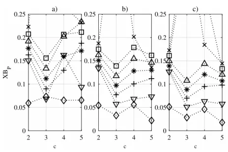
give sufficient information on the behaviour of clustering. The XB index was evaluated using these settings. The results are shown in Fig. 6, where the three diagrams show XBP as a function ofcwith varyingaweight at three differentm values. Subfigure a) was obtained with the smallest,m= 1.4 value, b) with the standard m= 2, and c) with the highest, m= 2.2 value. These were selected

510

only for illustration, as all the intermediate values show similar trends.

2 3 4 5

c 0

0.05 0.1 0.15 0.2 0.25

XB P

a)

2 3 4 5

c 0

0.05 0.1 0.15 0.2

0.25 b)

2 3 4 5

c 0

0.05 0.1 0.15 0.2

0.25 c)

Figure 6: XBP as a function ofcanda, at variedmvalues. a)m= 1.4 b)m= 2.0 c)m= 2.2

♦:a= 0.1,5:a= 0.4, + :a= 0.7,

∗

Comparing the three subfigures in Fig. 6, one can see that in most cases, the effect of the fuzzifier is small, as the XBP values follow similar trends in case of each m. This is in agreement with the findings of the previous study [19], and therefore the standard value ofm= 2 is accepted and applied in the

515

following.

By looking for the minimum of XBP, one can see that for moderate values ofaaround unity, ranging from 0.4 to 1.3, the optimal cluster number isc= 3.

These results are similar to those obtained with a non-periodic FCM in [19],

reproduced here in part a) of Fig. 8. For a = 0.1, the minimum of XBP is

520

found atc= 5 for eachm, however, this should not be accepted as the optimum c, since XB has a tendency to have decreasing values asc increases, regardless of the goodness of clustering [32]. Furthermore, this is in contrast with the previously mentioned recommendation regarding√

N being the largest number of clusters to be considered. Therefore such high c values should be treated

525

with criticism. For values of a = 1.6 and higher, XBP again often reaches its minimum at c = 5, but similarly to the previous case, this should not be considered as the optimum c. In these cases, the real optimal cluster number is probablyc = 2. These aare significantly larger than unity though, and the clustering results with these settings differ substantially from those obtained

530

witha≈1, therefore they should not be accepted.

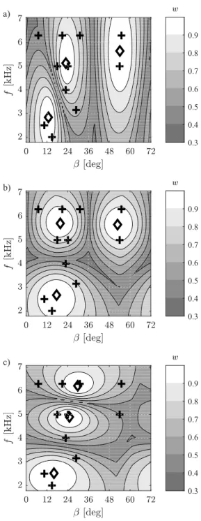
The way a transforms the results is shown in Fig. 7. There the cluster maps can be seen for various a= 0.1, a= 1, and a= 1.9 values, with c = 3 and m = 2 fixed. For lower values of a, the clusters are elongated in the ˆf dimension, while for higher values, the opposite occurs, and the cluster extend

535

in the ˆβ dimension.

Based on Figs. 6 and 7, the optimal weight is a= 1. This is because this presents a good compromise between the elongation of the clusters along the two dimensions. Furthermore, around this value, in a fairly wide range ofa= 0.4 toa= 1.3, the value of XBP is stabilised and shows the theoretically expected

540

tendency, with a global minimum inside the range, e.g. not at the limits of the investigated c values, being independent of the choice of m. This a = 1 result means that ˆβ and ˆf are to be taken into account with equal weights, indicating the equal importance of spatial and frequency-wise extension of the noise sources.

545

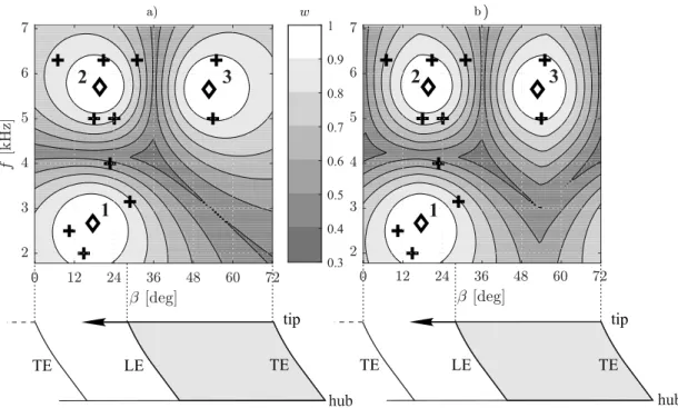
The optimal cluster number atR= 1.0 belonging toa= 1 isc= 3, according to Fig. 6. Therefore the cluster map with these parameters,m= 2,a= 1 and c= 3, was evaluated in detail, and compared to the cluster map obtained with the standard FCM algorithm in [19]. In the specific case study reported herein, the periodic and non-periodic methods have both led to c= 3 as the optimal

550

Figure 7: Cluster maps forc= 3 andm= 2 withavaried. +: data points,♦: cluster centres.

a)a= 0.1, b)a= 1, c)a= 1.9. The contour map shows the maximum membership value at each point.

cluster number. In general however, the introduction of periodic clustering may give results that are substantially different from those of the original FCM, as illustrated by Fig. 1.

AtR= 1.0, the periodic and non-periodic cluster maps are visually similar, shown in Fig. 8 as parts a) and b), respectively. There is some difference

555

due to the periodic clustering though. The membership contour-lines of the bottom-left cluster, termedCluster 1 in [19], extend through the edge of the diagram in case of periodic clustering. The membership iso-lines of the upper two clusters have a modified shape, as well, being compressed in theβ direction in the periodic case, compared to the non-periodic one. This is the result of

560

the periodicity being taken into account, as now these clusters influence each other both from in between them, and from the limits of the angular dimension, β = 0^◦ and β = 72^◦. The contour map shows the maximum membership value at each point. Thesewvalues have changed, too, and their contours have became continuous at the vertical edges of the diagram, due to periodicity being

565

accounted for.

The similarity between the two figures shows that intuitively assigning the trailing edge of the blade asβ= 0 was an appropriate choice. However, this was previously done based on a subjective visual evaluation, which is not required any more, when applying the periodic clustering method, since in the present

570

case, the results do not depend on the analysis window.

As the clusters have not changed significantly, their interpretation, given previously in [19], is still considered valid. Here, due to the nature of the spectrum shown in Fig. 4, only broadband source mechanisms were considered.

The identified mechanisms are summarised below. The cluster numbers refer to

575

those in Fig. 8.

• Cluster 1 represents the turbulent boundary layer – trailing edge interac- tion noise. There are three reasons leading to that conclusion [19]. First, Cluster 1 is in the vicinity of the trailing edge of the previous blade. Sec- ond, the frequency of this cluster centre, being about 2.8 kHz, is in fair

580

hub hub

Figure 8: Clusters forc = 3, m = 2 and a= 1. +: data points, ♦: cluster centres. a) standard FCM clustering b) the proposed hybrid clustering method. The contour map shows the maximum membership value at each point. The numbers indicate the cluster numbers.

At the bottom, the lines indicate the trailing edges (TE) and leading edges (LE) of the fan blades, together with the tip radius.

agreement with the peak frequency of this noise source, being about 1.2 kHz [35], especially considering that third octave bands below 2 kHz were not processed here. Third, the derivative of the beamforming level with respect to the frequency, which is about 7 dB/kHz, agrees fairly well to the 8.6 dB/kHz obtained from models related to this noise generation

585

mechanism [35, 36, 37].

• Cluster 2 represents thetip leakage flow noise. The reasons behind that are as follows. First, the location, being positioned between two blades.

Second, the frequency of the cluster, being about 5.8 kHz, agrees well with the frequency of 5.2 kHz reported for this source type in [35]. Furthermore,

590

the frequency derivative of the beamforming level, being 2.3 dB/kHz, and the shape of the beamforming level spectrum, is again in agreement with references [35, 38] that report a value of 2.2 dB/kHz for tip leakage flow.

• Cluster 3 represents the double leakage flow noise. This type of noise source originates from a tip leakage flow that that reaches the pressure side

595

of the adjacent blade around the tip region, where it leaks again, reaching the third blade [39]. The frequency of this cluster, and the frequency derivative of the beamforming level in this cluster is similar to those of Cluster 2, suggesting that the two sources are related. However, this is located further downstream from the trailing edge, when compared to

600

Cluster 2. This leads to the conclusion that Cluster 3 is related to the double leakage flow noise. Similar observations, supported by numerical and experimental fluid dynamics analyses, are reported in [13, 14, 15].

For more details on the analysis process, and for the reasons behind excluding further generation mechanisms, the Reader is referred to [19].

605

5.2. Comparative evaluation of multiple radii

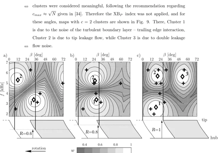
The same approach was applied onto the two remaining radii. As noted before, N = 5 and 7 base sources were identified after filtering at R = 0.6 and 0.8, respectively. Due to the small number of data points, only c = 2

clusters were considered meaningful, following the recommendation regarding

610

cmax ≈√

N given in [34]. Therefore the XBP index was not applied, and for these angles, maps with c= 2 clusters are shown in Fig. 9. There, Cluster 1 is due to the noise of the turbulent boundary layer – trailing edge interaction, Cluster 2 is due to tip leakage flow, while Cluster 3 is due to double leakage flow noise.

615

0.4 0.6 0.8 1

a) b) c)

rotation

R=0.6 R=0.8 R=1

tip

hub

1 1 1

2 2

2 3

Figure 9: Cluster maps. +: data points,♦: cluster centres. a)R = 0.6, b)R = 0.8, c) R= 1.0. β= 0 indicates the location of the trailing edge of the preceding blade atR= 1.0.

The shaded areas indicate the fan blades, which are not to scale, however, the lines showing the trailing and leading edges are placed according to their physical positions. windicates the maximum membership value at each point. Cluster 1: turbulent boundary layer – trailing edge interaction noise. Cluster 2: Tip leakage flow noise. Cluster 3: double leakage flow noise.

To provide further information relating to the maps at different radii,cluster amplitudes σwere introduced. The cluster amplitudeσi represents the strength of the source attributed to the i-th cluster. This is calculated as shown in Eq. (18), using the data point amplitudes pi, which were obtained from the Fourier expansion of the circumferential source strength distributions. As the

620

aim is to qualitatively compare the maps and not to quantify them, the exact values of cluster amplitudes are not reported, only their relation to each other, therefore the pi values are used in a dimensionless form. Cluster amplitudes were determined separately for each cluster and each radius.

σi=

N

X

j=1

wi,jpj (18)

As seen in Fig. 9, Cluster 1, connected to turbulent boundary layer – trailing

625

edge interaction noise, was identified at all radii. Its location is similar in all maps: the cluster centre is located about 20 degrees downstream of the trailing edge, following its inclination due to blade skew, and its frequency is around 3 kHz. This trend, i.e. that base sources positions follow the skewed trailing edge, is apparent in other maps, as well, from R = 0.5 throughout R = 1.0,

630

which are not shown here. The amplitude of Cluster 1,σ1was found to increase monotonically with increasing radii: atR= 0.6, it reached 27% of the amplitude at the tip radius, while atR= 0.8, this value was 62%. This may be connected to the spanwise increase of circumferential velocity and flow velocity. Therefore, the sets of Cluster 1 match the spanwise changes in trailing edge geometry and

635

in flow conditions.

Cluster 2 was is also found in Fig. 9, where its frequency is around 5.5 kHz in all three maps. Its location is consistently about 20 degrees downstream of the trailing edge atR = 0.8 and 1.0. This cluster was connected to the noise due to tip leakage (R= 1.0). Therefore, Clusters 2 ofR= 0.8 andR= 0.6 are

640

considered as the weakened signatures of the tip leakage flow appearing at these lower radii, as well, due to the limited spatial resolution of the beamforming technique. This view is supported by the fact that theσamplitude of Cluster 2 decreases monotonically towards the hub: atR= 0.8, 54% of the amplitude was found, while atR= 0.6, it was about 19%. The limit in spatial resolution

645

causes a variance in the angular position of Clusters 2, as well.

AtR= 1.0, Cluster 3 was found, as well, and it was connected to the noise of double leakage flow. At lower radii, this cluster was not found. This is

attributed to the limited spatial extent and strength of the double leakage flow.

In summary, three clusters were localised in the rotor annulus. These are

650

in good agreement with those found earlier in [19], which represent turbulent boundary layer – trailing edge interaction, tip leakage, and double leakage noise.

The clusters at the different radii are physically related, are found at similar frequencies, and mostly follow the shape of the skewed trailing edge.

6. Conclusions

655

A new method was presented for the fuzzy clustering of data points in a hybrid data set. Its advantage is being able to identify clusters in a periodic feature space, regardless of the number of total dimensions. It can only be applied however, if there is exactly one periodic dimension.

Application of the algorithm was illustrated in a case study to investigate

660

noise sources in axial fans, by analysing beamforming maps. For the sake of robustness, sensitivity studies were carried out to determine the parameters.

The number of clusters was found with the help of the extended XB index, taking periodicity into account. The effect of fuzzifier was investigated, and in the present case study, was found to have little influence on the results in the

665

usually suggested range. The relative importance of the different dimensions was evaluated as well, again through a parameter study, to find the optimal weights for the distance measure. These sensitivity studies onm and ak, also in determiningcvia the XB index, are recommended on a case-specific basis in every case for which the method is applied.

670

The procedure was carried out for multiple radii on the blade surface, in order to obtain spanwise information about the noise sources. The clusters of turbulent boundary layer – trailing edge interaction noise were found to be in accordance with the spanwise change in blade geometry and in velocity condi- tions. The clusters of tip leakage flow were noise also appeared at radii further

675

away from the tip, drawing attention to limitations in spatial resolution of the applied beamforming technique.

The results show that the proposed beamforming map analysis method is robust, and the parameter sensitivity study provides objective choices for the variables. Thus, it allows the analysis of beamforming maps in a concerted and

680

objective way, allowing researchers to identify the dominant noise sources being present in an axial fan. The periodic clustering method is however not restricted to beamforming or fan data, and could see a wide range of applications.

Acknowledgements

The authors thank Tam´as Kalm´ar-Nagy for his useful suggestions regarding

685

the distance metric.

This work has been supported by the Hungarian National Research, Devel- opment and Innovation Centre under contract No. K 112277.

The research reported in this paper was supported by the Higher Educa- tion Excellence Program of the Ministry of Human Capacities in the frame of

690

Water science & Disaster Prevention research area of Budapest University of Technology and Economics (BME FIKP-V´IZ).

References

[1] R. P. Dougherty, Beamforming in acoustic testing, in: T. J. Mueller (Ed.), Experimental Aeroacoustics, Springer, Berlin, 2002, pp. 62–97. doi:10.

695

1007/978-3-662-05058-3.

[2] L. Koop, Beamforming in acoustic testing, in: M. L. Riethmuller, M. R. Lena (Eds.), VKI Experimental Aeroacoustics, von K´arm´an In- stitute for Fluid Dynamics, Rhode Saint Genese, 2006. doi:10.1007/

978-3-662-05058-3.

700

[3] E. Balla, J. Vad, Establishment of a beamforming dataset on basic models of low-speed axial fan blade sections, Periodica Polytechnica, Mechanical Engineering 61 (2) (2017) 122–129. doi:10.3311/PPme.9548.

[4] P. Sijtsma, S. Oerlemans, H. Holthusen, Location of rotating sources by phased array measurements, in: Proceedings of the 7^th AIAA/CEAS

705

Aeroacoustics Conference, Maastricht, 2001. doi:10.2514/6.2001-2167.

[5] G. Herold, E. Sarradj, Microphone array method for the characterization of rotating sound sources in axial fans, Noise Control Engineering Journal 63 (6) (2015) 546–551. doi:10.3397/1/376348.

[6] R. Dougherty, B. Walker, Virtual rotating microphone imaging of broad-

710

band fan noise, in: 15th AIAA/CEAS Aeroacoustics Conference (30th AIAA Aeroacoustics Conference), 2009, p. 3121. doi:10.2514/6.

2009-3121.

[7] W. Pannert, C. Maier, Rotating beamforming–motion-compensation in the frequency domain and application of high-resolution beamforming al-

715

gorithms, Journal of Sound and Vibration 333 (7) (2014) 1899–1912.

doi:10.1016/j.jsv.2013.11.031.

[8] G. Herold, F. Zenger, E. Sarradj, Influence of blade skew on axial fan component noise, International Journal of Aeroacoustics 16 (4-5) (2017) 418–430. doi:10.1177/1475472X17718740.

720

URLhttps://doi.org/10.1177/1475472X17718740

[9] F. Zenger, G. Herold, E. Sarradj, Acoustic characterization of forward- and backward-skewed axial fans under increased inflow turbulence, AIAA Journal 55 (4) (2014) 1241–1250. doi:10.2514/1.J0555383.

[10] F. Kr¨omer, J. M¨uller, S. Becker, Limitations of phased array beamforming

725

in open rotor noise source imaging, AIAA Journal 56 (4) (2018) 1507–1518.

doi:10.2514/1.J056324.

[11] O. Minck, N. Binder, O. Cherrier, L. Lamotte, V. Budinger, Fan noise analysis using a microphone array, in: International Conference on Fan Noise, Technology and Numerical Methods (Fan 2012), Senlis, 2012.

730

[12] F. J. Zenger, G. Herold, S. Becker, E. Sarradj, Sound source localization on an axial fan at different operating points, Experiments in Fluids 57 (8) (2016) 136. doi:10.1007/s00348-016-2223-8.

[13] T. Benedek, J. Vad, Study on the effect of inlet geometry on the noise of an axial fan, with involvement of the phased array microphone technique, Pa-

735

per ID GT2016-57772, in: Proceedings of ASME Turbo Expo 2016, Seoul, 2016. doi:10.1115/GT2016-57772.

[14] T. Benedek, J. Vad, An industrial onsite methodology for combined acoustic-aerodynamic diagnostics of axial fans, involving the phased ar- ray microphone technique, International Journal of Aeroacoustics 15 (1-2)

740

(2016) 81–102. doi:10.1177/1475472X16630849.

[15] T. Benedek, J. Vad, Spatially resolved acoustic and aerodynamic studies upstream and downstream of an industrial axial fan with involvement of the phased array microphone technique, in: Proc. 11^th European Conference on Turbomachinery Fluid Dynamics and Thermodynamics, Madrid, Spain,

745

2015.

[16] P. Sijtsma, CLEAN based on spatial source coherence, Interna- tional Journal of Aeroacoustics 6 (4) (2007) 357–374. doi:10.1260/

147547207783359459.

[17] T. F. Brooks, W. M. Humphreys, A deconvolution approach for the

750

mapping of acoustic sources (DAMAS) determined from phased micro- phone arrays, Journal of Sound and Vibration 294 (4) (2006) 856–879.

doi:10.1016/j.jsv.2005.12.046.

[18] B. T´oth, J. Vad, Fourier analysis of beamforming data at the tip of an axial fan rotor, Periodica Polytechnica, Mechanical Engineering 60 (3) (2016)

755

152–158. doi:10.3311/PPme.8935.

[19] B. T´oth, J. Vad, Algorithmic localisation of noise sources in the tip region