Climate change, impacts and responses
Mika, János
Climate change, impacts and responses
Mika, János
Publication date 2011
Szerzői jog © 2011 Hallgatói Információs Központ
Copyright 2011, Educatio Kht., Halgatói Információs Központ. Felhasználási feltételek
Tartalom
1. Climate change, impacts and responses ... 1
1. R_1.1 Education of geography by climate change ... 1
2. R_1.2 Weathering: a complex effect of climate ... 4
3. R_1.3 Developing the key competences ... 5
4. R_1.4 Refreshing the other school subjects ... 7
5. R_1.5 Practical aspects of climate ... 7
5.1. R1.5.1 Weathcer extremes ... 8
5.2. R1.5.2 Low-energy, low-carbon life ... 8
6. Atmospheric variables ... 9
7. 1.2 Further components of the climate system ... 11
8. 2.1 Changes in the radiation balance ... 16
9. 2.2 Recent results on the greenhouse gases ... 18
10. 2.3 Observation of aerosol concentrations ... 19
11. 2.4. Effects of land use ... 20
12. 2.5 Greenhouse gases and other problems of air chemistry ... 21
13. 3.1 Attribution of the changes ... 22
14. 3.2 Comparison with the last 1000 years ... 24
15. 3.3 Capability and limitations of the present climate models ... 24
16. 3.4 Testing of climate reproduced by models ... 26
17. 3.5 Testing climate model sensitivity ... 27
18. 4.1 Projection of the global mean warming ... 28
19. 4.2 Patterns of climate change ... 30
20. 4.3 Reality of a jump-like glacial climate ... 33
21. 5.1 Projections for Europe by GCMs ... 34
22. 5.2. Inter-model variability of pressure changes: uncertainty for mezo-scale models ... 35
23. 5.3 Results of regional climate modelling ... 37
24. 5.4 Empirical comparison of regional vs. global changes ... 38
25. 5.5 Effects of land use in Hungary (after Drüszler et al., 2010) ... 40
26. 6.1 Damages from the extreme meteorological events ... 42
27. 6.2. Extremes of present climate ... 43
27.1. 6.2.1 Weather extremes ... 43
27.2. 6.2.2 Significant circulation objects ... 45
27.3. 6.2.3 Climate extremes ... 46
28. 6.3 Spatial distribution of weather and climate extremes ... 48
29. 7.1 Expectations on changes in the extremes ... 49
29.1. 7.1.1 Statistical considerations ... 49
29.2. 7.1.2 Physical considerations ... 50
30. 7.2 Data quality, free oscillation and conceptual problems ... 51
30.1. 7.2.1 The data problem ... 51
30.2. 7.2.2 The free oscillations problem ... 52
30.3. 7.2.3 Conceptual problems ... 52
31. 7.3 What is seen from the data? ... 53
31.1. 7.3.1 Temperature extremes ... 54
31.2. 7.3.2 Precipitation extremes ... 55
31.3. 7.3.3 Wind extremes ... 55
31.4. 7.3.4 Tropical cyclones ... 57
32. 8.1 Definitions of drought ... 58
33. 8.2 The Palmer Drought Severity Index ... 58
33.1. 8.2.1 Principle and computation of PDSI ... 58
33.2. 8.2.2 Correlation of PDSI with soil moisture estimations ... 59
33.3. 8.3 Can the drought be a consequence of greenhouse warming? ... 60
34. 9.1 Impacts of global warming in the different climatic belts ... 62
35. 9.2 Vulnerability and adapting capacity of the various sectors ... 65
36. 9.3 Geographical Analogy – Links to Some Hungarian Scenarios ... 67
37. 9.4 Impacts on natural vegetation: Renaissance of an old diagram ... 69
38. 10.1 Concentrated efforts on climate impacts in Hungary ... 70
38.1. 10.1.1. Climate and extremes in Hungary ... 70
38.2. 10.1.2 Basic results and recommendations of the VAHAVA project ... 71
38.3. 10.1.3 The National Climate Change Strategy ... 72
38.4. 10.1.4 Follow-up activities related to impact research ... 72
39. 10.2 Impact in Hungary – selected aspects ... 73
40. Wheat yield ... 79
41. 11.1 Weather relatedness of the tourism business ... 79
42. 11.2 Climate change and tourism ... 81
43. 11.3 Bioclimatic indices of the thermal environment (after Németh Á., 2008) ... 82
44. 11.4 Adaptation of tourism to the weather and climate extremes ... 84
45. 11.5 Consequences of a global warming on sea level ... 84
46. 12.1 The minimum goal: to avoid jump-like climate changes ... 85
47. 12.2 Possibilities of mitigation ... 86
1. fejezet - Climate change, impacts and responses
R_1 Education of geography by climate change (Reading)
Climate change and related aspects are of concern even for the youngest generation. This fact may be a good starting point to emphasise some related aspects of science and of society. Many aspects were just dead subjects for our pupils without this enhanced attention.
Climate change is an exciting scientific and practical challenge of our era. Acting today in this regards yields positive results for the next generation. This is why young generation should also be involved into these pieces of knowledge to motivate them for contributing to focused response of society in mitigation of the changes and in adaptation to them. In preparation of these tasks geography undertakes a key role from among education subjects.
Though science is still engaged with several questions to explain the past trends and with even more to project the future, there are some very likely statements which can be used as a basis for education of and by climate change. They are, at least, the following ones:
1. Anthropogenic origin of the recent global warming is very likely (i.e. >90 %, IPCC, 2007). No better news occurred ever since (The Copenhagen Diagnosis, 2009).
2. The warming should be as early as possible, but by all means before 2 K compared to the initial state to avoid unmanageable critical jumps. There are many opportunities for that but none of them is cheap or surely more effective, than the other ones.
3. Impacts of the changes vary regionally and the adaptation needs also regional research and planning. The extremes do not universally become more frequent, or more rapid, but we must gradually adjust our concepts and thresholds.
The above statements may change from time to time, as science evolves. Climate change means a life-long challenge for teachers to be well informed when contacting the students.
1. R_1.1 Education of geography by climate change
Last, but not least geography, as the probably closest subject to the climate change issue. Geography is not less complex, than biology, since it includes not only living and lifeless spheres of the earth, but also the society, as it is indicated by the image. On the other hand geography, as it follows from its name, first describes its discipline in widest complex approach, but it does not surely want to solve every detail, since single topics of geography often form limited, but infinitely deep individual disciplines.
Geography is a so called chorological science (chorology: study on distribution, in ancient Greek), i.e. it investigates the geo-systems. Geo-systems are systems of the common space of natural and societal interactions among the solid (lithosphere), fluid (hydrosphere), gaseous (atmosphere) and living (biosphere) sub-systems.
This space of interaction is called geo-sphere, geographical shell or geographical environment. The main branch of geography is physical geography, dealing with the natural processes and interactions of the environment. A key term of this branch is the landscape, sometimes bearing regional character. The other main branch is tie social or human geography, sometimes also called economical geography, dealing with interactions of landscape and society or various aspects of society with each other. As it is seen in Fig. R1.1, physical and social geography are not always separated. They are mainly connected by the common space filled by both of them and the need for holistic view and application of results from both branches for the wealth of society.
Figure R1.1. Main branches of physical and of social geography with their interaction. (Source:
http://www.physicalgeography.net/fundamentals/1b.html)
Geography studies the systems of the common space of natural and societal interactions among the solid (lithosphere), fluid (hydrosphere), gaseous (atmosphere) and living (biosphere) spheres. This space of interaction is called geo-sphere, geographical shell or geographical environment. Solid shell of the earth is rather popular among the pupils since one can collect its products even by their free hands. Geography embraces the organised co-existence of people in many aspects. Most straightforward among them are the Economical geography and Social Geography. Some key aspects of these fields, indicated in the table, can also be emphasized for themselves, also in relation with the changing climate. Examples for using the climate change for developing various aspects of geography are listed in Table 4.
Table R1.1 Examples of geographical phenomena related to climate with some explanations.*
Phenomenon/process Broader topic Reason for emphasis Relation to climate
Rea-arrangement of population distribution.
Migration, over-
population conflicts.
Population Geography Requirements to sustain in a region, correlation of population and natural resources.
Critical changes, e.g.
desertification, loss of Himalaya glaciers.
Transformation of the settlements. Over- population in the mega- cities.
Settlement Geography Requirements to establish and to sustain a settlement.
Cross-cutting of climate
warming and
overpopulation.
Polar ecosystem reduction Sea-level (volume) rise Changes in flooding frequency
Loss of drinking water in the Himalaya region
Hydrology (Hydro- geography)
Vulnerability of sea-ice and mountain glaciers.
Processes to influence the sea level. Climatic & other causes of flood.
Warming fast at the poles.
Expansion, melt of pack ice.
More intense rains, heat- waves.
Shift of vegetation zones;
extinction of species, expansion of other species.
Biogeography Importance to retain the present biodiversity.
Possibilities and
Regional climate changes, reminding to shift of climate zones.
Expansion or reduction of the wet ecosystems.
limitations of the vegetation to adapt.
Spontaneous and managed adaptation to the climate changes, possible modification of its extremes.
Occurrence of new pests.
Agricultural Geography Possibilities & limits of biological adaptation.
Effect of environment on the competition among the species. Adaptation by plant breeding.
Slow changes, but changes in extreme events.
Economic effect of the climate changes: costs of adaptation and mitigation.
Economic Geography Showing the costs (and incomes) of selected key economical activities.
Slow changes, but changes in extreme events.
Changes in water, road- and rail connections partly related to primary (drying) and secondary (settlement structuring) reasons.
Transportation Geography Factors determining water- , road or rail connection
(including the
environmental conditions, as well).
Consequences of climate change in water levels, their stability and on population.
Lack of food and water, poverty, epidemic
Social Geography Existence and
geographical distribution of poverty, famine, thirst and epidemic.
Slow changes, but changes in extreme events.
Physical changes of the natural surfaces
Geology Rock disintegration in the process of weathering (rain, ice, wind, temperature)
Extreme weather
conditions, likely more intense with warming.
Soil erosion
Slow shift of the zonal and non-zonal soil types
Pedology (Soil
Geography)
Process and consequences of soil degradation.
Intensive rains, likely more frequent with the warming.
*The author is thankful to Dr. Ilona Pajtok-Tari for collecting this table for another study (Pajtok-Tari I. et al., 2011)
A pair of further disciplines of human geography is even more directly affected by climate, though they are influenced by other trends of population and other sources of stresses. From time to time, even the climate anomalies (i.e. long-term, weather extremities) can cause faster (but more recoverable) versions of the longer- term threats.
During one generation the sea ice area did dramatically shrink in the Northern Hemisphere. It is also a good point to call the pupils attention on why the Southern Hemisphere does not suffer from the same rapid changes.
This is a fairly old pair of figures, so one may also call the pupils to find much more recent figures on the same topic.
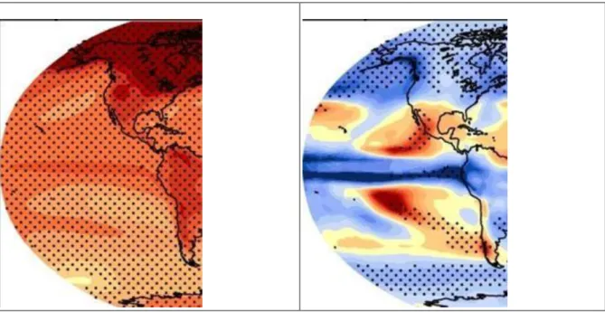
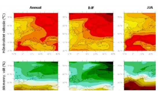
Zonality and continental differences are obvious features of our present climate. They reflect different physical characteristics of the solar radiation and heat capacity of various domains of the climate system. Are these differences markedly reflected by the patterns of past and future climate changes, too? The answers to this question are illustrated by seasonal changes of temperature and precipitation in Fig. R1.2 (also demonstrated and analysed in Chapter 4) taken from the IPCC WG-I (2007) Report. They are averaged for all available models, i.e. they are results of pure physics. As such, they are concentrated illustrations of several phenomena used in physical geography. Analysis of these changes is an impressive tool to demonstrate zonality and continentality, these key aspects in education of physical geography.
Figure R1.2. Model-mean changes of temperature (warming) and precipitation (different signs).
These key aspects of geography are:
1. Zonality of the changes, clearly seen both in temperature and precipitation. The strongest changes near the pole are characteristic features of the changes due to the ice/snow–albedo feedback changes. The belts of precipitation changes, due to circulation reasons, are also present in the differences of both variables and seasons. However, combined effects of these variables on runoff or soil moisture changes are already influenced by effects of non-zonal topography and soil taxonomy.
2. Continentality is seen both in the faster changes of the temperature over the continents, and in the slower changes on the west coasts. In the precipitation fields, this term is seen in the summer half year of both hemispheres as a disturbance of the zonal structures. Another feature of continentality is that the Northern Hemisphere, covered by continents to larger extent, warms faster parallel to the global changes.
2. R_1.2 Weathering: a complex effect of climate
Weathering is the process of disintegration of rock from physical, chemical, and biological stresses. I.e. this is one of the processes in our Planet which can well be explained in each of the four natural sciences, physics, chemistry, biology and geography. Weathering is influenced by temperature and moisture (climate).
The degree of weathering that occurs depends upon the resistance to weathering of the minerals in the rock, as well as the degree of the physical, chemical, and biological stresses. A rule of thumb is that minerals in rocks that are formed under high temperature and pressure are less resistant to weathering, while minerals formed at low temperature and pressure are more resistant to weathering. Weathering is usually confined to the top few meters of geologic material, because physical, chemical, and biological stresses generally decrease with depth.
Weathering of rocks occurs in place, but the disintegrated weathering products can be carried by water, wind, or gravity to another location.
Figure R1.3 indicates how temperature affects weathering in our present climate.
Figure R1.3: Influence of the interaction of temperature and rainfall on processes of physical and chemical weathering. As annual rainfall and temperature increase, chemical weathering dominates over physical weathering. On the contrary, notice that as the temperature lowers, physical weathering begins to dominate over chemical weathering. Image courtesy of University of Nebraska–Lincoln, 2005. http://plantandsoil.unl.edu/crop technology2005/soil_sci/?what=topicsD&
informationModuleId=1124303183&topicOrder=2&max=7&min=0&
3. R_1.3 Developing the key competences
Modifying tasks of education, as developing the competences becomes also important, besides knowledge transfer. The revision of National Core Curriculum (NCC) in 2003 and 2006-2007 pointed at importance of developing the so called key competences, besides the topical requirements what the pupils should own as knowledge. The key competences became core parts of the NCC. These are outstandingly important abilities, which are inevitable to further learning and to successful participation in the society and world of labour. These competences in Hungary are based on those elaborated by the EU (ERF, 2007).
The nine key competencies are the followings (NCC, 2007) 1. Communication in the Mother Tongue
2. Communication in Foreign Languages 3. Mathematical Competence
4. Competences in Natural Science 5. Digital Competence
6. Learning to learn
7. Social and Civic Competences
8. Sense of Initiative and Entrepreneurship
9. Aesthetic and Artistic Awareness and Expression
Table R1.2: Examples on how climate change can be used to improve the key competences
Key competence (KC) Example of using climate change to develop the KC
Communication in the Mother Tongue
1. learn new words of climate, effects and responses
Communication in Foreign Languages
1. find extra motivation in understanding the CC disputes
Mathematical Competence
1. use CC as motivation to understand usefulness of math
Competences in Natural Science
1. use CC to teach and integrate Natural Sciences
Digital Competence
1. besides the Internet, compilations and calculations in CC
Learning to learn
1. use CC as a fast developing topic to learn for learning
Social and Civic Competences
1. weather extremes are good examples of cooperation
Sense of Initiative and Entrepreneurship
1. renewable- and low-carbon industry are good examples
Aesthetic and Artistic Awareness and Expression
1. nature itself provides picturesque examples in storms
Table R1.2 provides a first-approach list on the possibilities to improve these competences by using the events, explanations and attitudes related to climate changes. In some cases the enhanced interest in weather and climate makes it more efficient in the circle of pupils and teachers, as well. For example, the lively discussion on the anthropogenic vs. natural origin on one hand, and the exciting news on extreme weather catastrophes, as well as
new possibilities to mine oil from below the Arctic-ocean may be worth reading in English or other languages even spontaneously, without classroom forcing, too.
One must admire that there is no specific key competence for environmental awareness. Causing less harm to the environment and delimiting other people and enterprises to pollute environment where it would be avoidable requires several other key competences. They are Competences in Natural Science, Social and Civic Competences, Aesthetic and Artistic Awareness at least, but maybe also the Expression Sense of Initiative and Entrepreneurship. We may surely state that climate change is a part of reality in the World around us. This means its global character, vast assortment of related phenomena and the common concern of majority of people (and mediums) made the problem widely appreciated among the pupils.
4. R_1.4 Refreshing the other school subjects
The school subjects can be refreshed in several respects, even if considering just the renewable energy (Table R1.3), as one single aspect of the whole climate change issue. There is no space to explain the examples, but please pay attention to the major challenges, and try to think through in your educational environment.
Table R1.3: Selected examples proving usefulness of the main school subjects,focused to (limited by) the renewable energies.
Subject Example of usefulness in the subject
Mathematics economical math, decision matrices, risks,
geometry (cline of solar collectors), etc
Physics material sciences (solar cells, wind rotors, etc.)
solution of energy accumulation, etc.
Chemistry bio-energy formation and utilisation,
save the devices from corrosion, etc.
Biology optimize for green mass (instead of e.g. grain mass)
recognition of bird flies in wind energy industry, etc.
Informatics automatic switches to alternate the energy sources
information mining (competing business!), etc
Geography spatial distribution of the energy sources, inc. biomass
role of societal structure and financial ability in the location
5. R_1.5 Practical aspects of climate
The climate change subject provides good opportunity to present the related problems of the environment, stemmed from the same anthropogenic over-consumption of the natural resources. This last subject claims for integration of these moments into long-term tasks for the whole society. There are two aspects which can not be expressed in detail due to space limitations, but which are important connections between school and everyday life. They are (i) the intelligent adaptation to weather, as ever-changing risk and resource for everyone and everywhere; and (ii) the energy-conserving way of life in our homes, including motivations for using renewable
energy. Both topics are good examples on those cases when fresh knowledge of the youngsters can guide the elder generation. (One should note, however, that the weather extremes are not direct consequences of climate change.)
5.1. R1.5.1 Weathcer extremes
Weather extremes are often quoted as rare, or intense event, but in some other cases those of high impacts. All three aspects are worth mentioning in education of the youngsters. By definition, the characteristics of what is called ―extreme weather‖ may vary from place to place. Specific concern at the middle latitudes is caused by thunderstorms, tornadoes, hail, dust storms and smoke, fog and fire weather. These small-scale severe weather phenomena range from minutes to a few days at any location and typically cover spatial scales from hundreds of meters to hundreds of kilometres. These extremes are accompanied with further hydro-meteorological hazards, like floods, debris and mudslides, storm surges, wind, rain and other severe storms, blizzards, lightning. For example, mudslides disrupt electric, water and gas lines. They wash out roads and create health problems when flood water spills down hillsides. Power lines and fallen tree limbs can be dangerous by causing electric shock.
Alternate heat sources used improperly can lead to injury from fire or carbon monoxide poisoning. The longer- term, precipitation- and temperature-driven set of extremities contain drought, wild-land fires, heat-waves, melting of permafrost and occurrence of snow avalanches, etc. Ca. 90 % of the natural disasters are somehow related to weather, concerning their material harm. Only the volcanic eruptions and the earthquakes are free of atmospheric forcing factors. These weather damages destroy over 10 % of gross domestic product in the poorest countries of the world (WMO, 2006). This number is ca 2 % in the richest countries (In Hungary it is just 1 %, due to its favourable geographical location in this respect.).
It is often possible to predict the probability of severe weather events quite accurately, issuing warnings, or closing the endangered regions, temporarily. The teachers must know the local signs of danger and respect warnings or prohibitions to enter the endangered areas. It is also possible to enhance rational awareness of the pupils against weather events to discuss the events of the recent past with them, either personally experienced or reported by the media.
5.2. R1.5.2 Low-energy, low-carbon life
Considering the extremity in global scale, we should establish that there are so called tipping points, where our climate may exhibit irreversible changes. Melting of the West Antarctic ice sheet, slow-dawn of the Atlantic thermohaline circulation and the El Nino – Southern Oscillation all may turn into a new state after 3 K of global warming (see in Ch. 12).
To avoid the 3 K warming the mankind must start decreasing its greenhouse gas emission by 2020, the latest.
This can be established by considering the so called policy-scenarios with the conclusion that the concentration should be stopped at 445-490 or 495-535 ppm equivalent CO2 concentrations. (This is a value when all greenhouse gases express the same forcing, as the CO2 in the given concentration.) Since this is a very complex question, majority of the mitigation requests consider 2 K for the maximum allowed warming for the future. Of course, the teachers can not be the key persons, who should achieve these mitigation targets. But, to know the main principal possibilities, such as renewable energy sources, nuclear energy (though considering its other environmental constraints), carbon sequestration, forest sinks etc., and to show the proper ways to support the reduction of last two components in the households and on the roads is our key role, in this respect.
* * *
In the above Sections we tried to demonstrate how meteorological facts, together with Internet-based- and traditional efforts to introduce climate-related knowledge and attitudes into the curricula, could increase the interest of present students and prospective teachers towards this set of questions as a part of the sustainable development. Too many and too dangerous extreme events occur, even without any climate change. It is worth knowing them and their harm for the teachers, and also listening to the forecasts. The alternatives to limit the greenhouse gas emission are also worth knowing in the school and performing in live at home. A key possibility of is to use renewable energy even if the fossil forms are still available. Mankind overcame the stone-age before running out of stones!
Scientific background (1-5 chapters)1. Observed changes of climate
The climate of our Planet has never been strictly constant, but the recent changes are by two orders of magnitude faster than the natural changes since the appearance of anthropogenic influence. The near surface air
temperature, which increased as much as 0.8°C in the last 100 years (Copenhagen Diagnosis, 2009). The temperature of the second part of 20th century on average was very likely above all 50 years in last 500 year‘s, and likely even in the last 1300 years. This fact and the realization of the likely reasons for the changes, plus rapid development of computer technology have resulted in systematic investigations of climate science.
Near-surface temperatures are, however, generally influenced by various local disturbances (developing cities, vegetation), modifications in the observation technology (changes of time, instrumentation or shading devices) or simply relocation of the weather (climate) station. Local temperature series may therefore be often non- homogenous which may disturb even the global reconstructions. Therefore, it is worth examining time series of other environmental parameters, related to climate.
6. Atmospheric variables
In this point we present the variation of observed climate of the world with the help of some typical graphs and maps. Variations of the near-surface temperature of the Earth as well as of the individual continents will be presented by the yearly averages of temperature in Point 2.2. Here we depict these temperature trends of the four seasons in the 1979-2005 time period (Fig. 1.1), as well, as the variation of temperature with the altitude (Fig.
1.2).
From top to down in Fig. 1.2, it is noticeable that the stratospheric temperature is decreasing. Considering that the increase of the greenhouse gases allows less energy to the stratosphere as before, we can already understand the temperature decrease. Furthermore, another reason contributes to this behaviour. It is the consequence of surface warming which leads to elevation of the tropopause and its lower temperature. This is the same process that leads to higher and cooler tropopause in summer than in winter.
Figure 1.1 Linear trends of surface temperature (K/10 yr) in the 4 seasons (marked by initials of the months).
Sign + emphasizes the areas where the trend is significant at the 95 % level. (Source: IPCC 2007: Fig. 3.10)
Figure 1.2 Global mean temperature of the air (in the respective order from A to D) in the stratosphere, in the upper troposphere, in the lower troposphere and near the surface. The two upper layers are derived from satellites‘ microwave sounding, the third one is a mixed series derived from satellites and radio-sounding measurements, while the lower level is based on the surface measurements. All anomalies are compared to the 1979-1997 mean values. The stratosphere is getting cooler, because the energy absorbed by the increasing amount of greenhouse gases is missing from the energy balance of these layers. Another reason is that the warming raises the level of the tropopause. (Source: IPCC, 2007: Fig. 3.17)
The temperature of the upper and lower troposphere, and also of the near-surface level shows encouraging synchrony. It is important because we can (unfortunately) exclude the hypothesis that the near-surface warming is just a result of measurement errors, or of erroneous neglecting of urban influence caused by large number of urban stations, since this effect would be much more localized in its vertical extent, as well.
We deal with other climate indicators in the followings, not tackling the sea level and the snow cover here, since these two quantities are demonstrated also in point 1.2. Firstly, in Fig. 1.3 we may see the global mean precipitation of the continents, which varies asynchronously with the global mean temperature.
Figure 1.3 Anomalies of precipitation of the continents in 1900-2005 in global average compared to the 1981- 2000 reference period, according to various authors' reconstructions. The solid curves are ten years‘ moving
averages. The main reason of the differences is that is that precipitation is distributed very patchy also in space.
Hence, differences of the station networks may influence the results. (IPCC 2007: Fig. 3.10)
Figure 1.4 Variations of the Palmer Drought Severity Index (PDSI) between 1900 and 2002 above the continents (upper graph). The red and orange colours indicate the drying of the upper layers of the soil, whereas the green and blue ones mark their becoming wetter. The global mean (lower graph) shows general drying, primarily due to the rise of temperature enhances the evaporation. (IPCC 2007: FAQ 3.2, Fig. 3.1)
From these one can establish that the globally averaged precipitation did not follow the variations of global mean average of temperature. But, this cannot even be expected, since precipitation is developing in rather complex macro- and mezzo-scale atmospheric objects, which vary rather differently in the various regions parallel to the global warming. The ca. 1000 mm/year global mean precipitation is distributed on the Earth rather unevenly. At the same time, the warming pushes the water balance of the upper soil layers towards the relative water shortage. (Figure 1.4)
7. 1.2 Further components of the climate system
The global mean near-surface temperature (observed in shadow at 2 metres above the surface) shows a 0.74 K warming between 1906 and 2005 (Figure 1.5). Within this, in the second 50 years the pace of the warming is ca.
its double, 0.13 K/decade. Likely, the northern hemisphere mean temperature of these 50 years is the warmest period over the last 1300 years.
Figure 1.5 Observed changes (a.) in the global average temperature, (b.) in the sea level, averaged globally according to the tide scales (blue), and the satellite data (red), as well, as (c.) in the area of snow cover of the Northern Hemisphere in the March-April period. The smoothed curves indicate the decennial averages, the circles show the decadal average values. All changes are compared to the 1961-1990 averages. The shaded areas show the uncertainty. (Source: IPCC WG-I, 2007.)
According to the recent investigations, unambiguous warming is established also in the upper and middle layers of troposphere, in coherence with the near-surface tendencies. This is essential, because in the previous IPCC Reports (1996 and 2001) this coincidence has not been yet established. An additional statement is that the maximum and the minimum temperatures contribute to the rise of the diurnal mean temperature in with identical weights. Warming of the oceans is already detected in its upper 3 km layer, which raised the sea level by 17 centimetres, already, together with warming of the continental ice sheets (Figure 1.5).
The total area of the mountain glaciers and the snow cover decreased in both hemispheres. The glaciers and the general decrease of the ice-caps contributed to the elevation of the sea level.
Table 1.1: The observed measures of the elevation of the sea level together with different factors that contributed to it. (IPCC, 2007: Decision Making Summary)
According to satellite observations, the annual mean expansion of the northern sea ice decreased by 2.7
%/decade since 1978. In summer this decrease is 7.4 %/decade! The upper layers of frozen soils (permafrost) in the Northern Hemisphere have been warming since 1980 by almost 3 K. The area of seasonally frozen soil decreased by ca. 7% in the Northern hemisphere since 1900, whereas in spring this number approaches the 15%!
From the start of the 20th Century precipitation has been growing unambiguously in Northern Europe, at the east coasts of the American continent, and in Asia's northern and middle regions. Climate became drier in the Sahel zone, and in the larger area of the Mediterranean Sea, as well, as in southern parts of Africa and Asia. The temporal distribution of precipitation developed unfavourably in two senses since both the duration of long dry (no precipitation) periods and amounts of individual heavy precipitation events have increased.
The temperate latitude general air circulation has also been modified in the recent 50 years parallel to changes of the sea surface temperature and in the area of snow cover. Important peculiarity of the change is the amplification of the temperate latitude west-eastern circulation on both hemispheres. Though, it is difficult to judge why it occurred, since the engine of the phenomenon, the meridional temperature gradient did definitely weaken in this period due to the faster than average warming of the polar and sub-polar regions.
Summing up 20th Century changes, we may establish that the mean air temperature of the northern hemisphere was very likely higher than any 50 year period over the last 500 years and likely warmer than any other one in the last at least 1300 years.
The warming (caused by anything) could be proven beside the air temperature with the change of other geophysical characters. Such variables are the area of snow cover and sea ice which could be detected well only in the era of satellites. Fig. 1.6 shows the changes of these components of the cryosphere in the last decades. As it is shown in the Figure both the snow cover and the sea ice area have decreased in the last decade parallel to the global warming over the Northern Hemisphere. Both changes are statistically significant.
Figure 1.6: The extension of snow cover on the continents of Northern Hemisphere in two following satellite observation interval during the thawing period, between 1967 and 1987, and 1988 and 2004 respectively (a).
The modification of snow cover represented by colour squares showing almost on every place 5-15 or 15-25%
shortening in time. The continuous lines are 0 and 5°C mean isotherms of air temperature for total 1967-2004 periods in March-April. The biggest area decreasing is nearly parallel with the isotherms. The next two figures show the extension of oceanic ice cover on the Northern (b) and Southern Hemispheres (c) between 1979 and 2005. The dots show the yearly mean ice extension, with decadal smoothing. (IPCC 2007: Fig. 4.3, 4.8 and 4.9).
On other hand, around Antarctica the sea ice has been increasing, despite the near-surface warming over the majority of the continent (Steig et al., 2009). This pattern has been attributed to intensification of the circumpolar westerlies, in response to changes in stratospheric ozone, letting less warm air masses into the centre of the island. This, in turn, leads to colder centre of Antarctica and southward shift of the Polar front.
In Fig. 1.6, the linear trend of ice cover decreasing is 33±7 thousand km2 per decade. Its magnitude is -2.7 %, and it is significant. Simultaneously, the ice-cover expansion, as much as 6±9 thousand km2 per decade, is not significant in the Southern Hemisphere.
Another indicator of the thermal processes is the sea level, driven mainly by the thermal expansion and the water balance with the continental ice. Sea ice melting does not influence the sea level, in correspondence with the Archimedes‘ principle on the floating objects.
Fig. 1.7 is evidence of warming showing the sea level rise combining the tide gauges and microwave satellite observations. The latter observations are based on the TOPEX/Poseidon and Jason satellite altimeter measurements programmes. They measure the sea level heights between 66°N and 66°S in ten-day averages since 1993. According to the processing of the measurements, the rise of sea level is 3.1±0.7 mm per year which mainly happens in the Southern Hemisphere.
Figure 1.7: Sea level change during 1970-2010. The tide gauge data are indicated in red (Church and White 2006) and satellite data in blue (Cazenave et al. 2009). The grey band shows the projections of the IPCC Fourth Assessment report for comparison. The graphs show the difference from the 1993 - June 2001 period‘s average in mm unit. The satellite data till 2002 are based on TOPEX/Poseidon, later on Jason satellites. (Copenhagen Diagnosis, 2009: Fig. 16)
Hence, the temperature increase has already been detected in the upper 3 km layer of the oceans. The reason is that 80% of the radiation balance surplus is absorbed by the oceans. (This is the 0.9 Wm-2 deviation of the total balance in Figure 6.1) This warming together with the thawing of land ice has already caused 17 cm elevation of sea level (IPCC, 2007).
According to the Copenhagen Diagnosis (2009), this increase of the sea level, its causes and the projected future can be summarised, as follows: The contribution of glaciers and ice-caps to global sea-level has increased from 0.8 mm/year year in the 1990s to be 1.2 mm/year today. The adjustment of glaciers and ice caps to present climate alone is expected to raise sea level by ~18 cm, (i.e. by 1 cm more after three years from 2005, than the IPCC AR4 estimation).
The area of the Greenland ice sheet, experiencing summer melt, has already been increasing by 30% since 1979, parallel to the increasing air temperatures. The net ice loss from Greenland accelerated since the mid-1990s and is now contributing as much as 0.7 mm/year to sea level rise due to both increased melting and accelerated ice flow.
Antarctica is also losing ice mass at an increasing rate, mostly from the West Antarctic ice sheet due to increased ice flow. Antarctica is currently contributing to sea level rise at a rate nearly equal to Greenland. Ice- shelves connect continental ice-sheets to the ocean. Signs of ice shelf weakening have been observed elsewhere than in the Antarctic Peninsula, indicating a more widespread influence of atmospheric and oceanic warming than previously thought.
There is a strong influence of ocean warming on the mass balance via the melting of ice-shelves. The observed summer melting of Arctic sea-ice has far exceeded the worst-case projections from climate models of IPCC AR4. The warming associated with the atmospheric greenhouse gas levels makes it very likely that in the later decades the summer Arctic Ocean will become ice-free, though the timing of this remains uncertain.
2. External forcing factors
Changes in global climate are forced by various processes that change the flows of radiative energy within the system. Either the absorption of solar radiation or the trapping of long-wave radiation by atmospheric constituents may change. Possible reasons for change include:
1. Change in solar irradiance or change in geometry of the Earth's orbit around the Sun.
2. Change in fraction of energy reaching the surface vs. the top of the atmosphere.
3. A change in the amount of outgoing (long-wave) energy at the top of the atmosphere.
These changes may occur due to both natural and man-made factors. The activity by which man can intervene in the atmospheric processes is changing the global energy balance of the atmosphere and the surface. This is possible in several processes.
Changes under headings 2.) and 3.), including both natural and man-made sources, may result from (i) Changes in the amount of long-wave radiation emitted by the surface and/or absorbed by various (the so called greenhouse-gases), cloudiness and H2O in the atmosphere; (ii) Changes in atmospheric transparency resulting from either variations in the amount of volcanic and anthropogenic aerosol in the atmosphere, or variations in cloudiness.
Changes in the forcing factors in the last 250 years are presented in Fig. 2.1. The most important conclusion, namely that the radiation balance of the Earth has been perturbed mainly by the greenhouse gases with some other changes worth also studying.
The effect of carbon-dioxide alone is approximately as strong during these centuries than the whole effect of all factors. This means that the warming effect of the non-CO2 greenhouse gases became fully compensated be
direct and indirect effects of the aerosols. The direct effect of aerosols means back-scattering of solar energy to the outer space.
The indirect effect means redistribution of the existing water content of the clouds from fewer large raindrops of larger diameter to increased number of smaller drops. The latter version created by the so called condensation nuclei, i.e. water solvable aerosols.
The greenhouse effect causes a general warming of the lower atmosphere and Earth's surface, and a compensating cooling of the upper stratosphere. The greenhouse gases of natural origin constitute main factors of the earth's climate: in the absence of water vapour, carbon dioxide and methane a climate of 33 K colder would dominate on our planet.
Danger of the climate modification effect of human activity is enhanced by the fact that most of the greenhouse gases have very long residence time. So, even if mankind decides to stop immediately all the activities that enhance the atmospheric greenhouse effect posterity would experience the consequence of previous releases even over centuries.
8. 2.1 Changes in the radiation balance
Carbon dioxide, however, is not the only one of the greenhouse gases whose amount increases owing to human activity. Just to mention the most important ones, they are the followings: methane deriving from rice paddies, live-stock breeding, biomass burning and the hydrocarbon industry; nitrous oxide that originates mainly from fertilisation and various fossil fuel combustion, moreover the halocarbons (species of freon and halon) widely used in the industry. The latter artificial gases have come into focus mainly because of their capability to dissolve stratospheric ozone.
Figure 2.1: Global mean radiative forcing (RF) estimates and uncertainty ranges in 2005 for anthropogenic carbon dioxide (CO2), methane (CH4), nitrous oxide (N2O) and other agents or mechanisms, together with the typical spatial scale of the forcing and the assessed level of scientific understanding (LOSU). The net anthropogenic radiative forcing and its range are also shown. Volcanic aerosols contribute an additional natural forcing but are not included in this figure due to their episodic nature. (IPCC, 2007: Fig. 2.20)
The most important greenhouse gases and the data on their concentrations and lifetime are listed in Table 2.1.
These gases generally absorb infrared radiation and thus contribute to the greenhouse effect of the atmosphere by reducing the amount of radiation emitted by the Earth's surface that escapes to the space. For this reason, such substances have come to be called 'greenhouse' gases.
Table 2.1: Present-day concentrations and the radiative forcing of the most important greenhouse gases. The changes since 1998 are also shown.
The observations clearly state that the atmospheric greenhouse-effect had increased since the industrial revolution. In accordance with what has been alleged and proven we can say that the anthropogenic greenhouse- effect is responsible for the significant part of the observed global temperature increase at least since 1900.
Based on reconstructed and measured data, we also know that the average temperature of the Northern Hemisphere slowly decreased in the last 1000 years with less certainly reconstructed and just partly understood long-term fluctuations (IPCC, 2007), until the beginning of 20th Century, with significant temperature increase afterwards.
Beyond the greenhouse effect and natural climate forcing processes (such as solar variability, changes is solar orbital parameters, volcanic activity), there are also further anthropogenic influences, i.e. the effects of sulfate aerosols, land cover change, stratospheric ozone depletion, black- and organic carbon aerosols and jet contrails, etc., with their various and partly non-negligible radiative effects. A comparison of these effects during the past 250 years is presented in the IPCC Report (IPCC, 2007)
Recently Trenberth et al. (2009) re-considered (Fig. 2.2) their earlier radiation balance estimations (Kiehl and Trenberth, 1997). The earlier period was based on observations from 1985 - 1989, whereas the recent estimates originated from March 2000 to May 2004 period. Very few terms of the radiation balance are unchanged during the 15 years. In some other cases the absolute difference between the two estimates is ca. 10 Wm-2, sometimes over 20 % in relative terms. The majority of the changes are likely caused by the uncertainty of the estimation, not the climate variation of the Earth during this period.
Figure 2.2: The annual mean energy budget of the Earth in the Mar 2000 - May 2004 period (Wm–2). The broad arrows indicate the schematic flow of energy in proportion to their importance. Source: Trenberth et al (2009) Remark: The Figure indicates global averages, independently from the type of the surface in the illustration.
Figure 2.3: Top panel: Compared are daily averaged values of the Sun‘s total irradiance from radiometers on different space platforms as published by the instrument teams since November 1978. Bottom panel: Sunspot number to illustrate the variability of solar activity for cycles 21, 22 and 23. (Source: Fröhlich, 2010)
E.g., Fig. 2.3 indicates that even the Solar constant varied by ca. Wm-2, which is comparable to the changes in the radiation balance due to most external forcing factors. In the latter period, near the maximum of the 23rd solar cycle, the incoming radiation was higher by ca 0.5 Wm-2 than in the previous period of the estimations, near and after the minimum between the 21st and 22nd cycles. However the instruments of the previous period gave a much stronger overestimation, leading to a -1 Wm-2 decrease of the Solar constant in the latter estimation.
The increasing of greenhouse effect modified the balance by 2.3 Wm-2 since the beginning of industrial revolution. The value is only 1% of the captured Sun originated energy but the 1/5 of the change has happened in the last decade. (The total energy balance remains zero at the top of the atmosphere, but it needs higher temperature near the surface, and above!)
Among the important anthropogenic forcing factors, the greenhouse effect influences the backward atmospheric long-wave radiation to the surface. (Its present value is 333 Wm-2, see above in Figure 2.2). The aerosol content modifies mainly the reflected short wave radiation (79 Wm-2) and, to a smaller extent, the atmospheric long wave emission (239 Wm-2).
Among the natural forcing factors, decadal oscillations of solar activity directly modulate the incoming short wave solar radiation (341 Wm-2), while the few bigger volcanic eruptions increase the reflected shortwave radiation 1-3 years. Changes of the mentioned factors will be briefly characterised in the following. The concentration of atmospheric carbon dioxide has grown from about 280 ppm before Industrial Revolution to 385 ppm in 2008 (Copenhagen Diagnosis, 2009). The methane concentration has grown from 0.715 to 1.774 ppm in 2005. Both values are much higher than any time in the last 650 thousand years! The atmospheric mass of similarly green house gas nitrous oxide has reached 0.319 ppm in 2005 from 0.270.
9. 2.2 Recent results on the greenhouse gases
The worldwide economical crisis led to -1.3% decrease in 2009‘s annual fossil-fuel CO2-emission (Fig. 2.4) comparing to 2008. One should note, however, that this 8.4±0.5 PgC emission is still larger by 37 % than that in
1990, considered as a reference in the mitigation policy calculations. The annual increase was as large as +3.2%
in the 2000-2008 period and for 2010 a >3% increase had recently been projected. (Global Carbon Project, 2010). The pace of the CO2-emission indicated in Fig. 2.4 was steeper than any IPCC (2007) scenario, compiled by Nakicenovic and Swart (2000)!
Natural land and ocean CO2 sinks removed 57% of all CO2 emitted from human activities during the 1958- 2009, each sink in roughly equal proportion. However, there is the possibility, however, that the efficiency of the natural sinks is declining. According to complex model calculations, the experienced decrease in both the biological and oceanic sources in the recent decades broadly explains this increase. The graph of the right side of Fig. 2.4 shows a dramatic increase of the airborne fraction is going on with increase of this fraction from 40%
to 45%.
The steeper than expected increase of the emission and the increased fraction of the emitted CO2 point at the possibility, that the present, post-IPCC (2007) estimate of the main greenhouse gas forcing is even more rapid than it was assumed by the Report in 2007! This increasing forcing is already seen in the global radiation balance, as presented in the next Section.
Figure 2.4: Trends in the fossil fuel vs. land-use forms of anthropogenic CO2–emission 1960-2009(left - Global Carbon Project, 2010) and the fraction of the emission remaining in the atmosphere
(right - Global Carbon Project, 2010)
The components of atmospheric aerosols have modified the atmospheric radiation balance in the opposite direction, namely decreasing the warming. The direct effect of aerosols, mainly the backscattering of solar radiation is about -0.5 Wm-2. Their indirect effect, through changes in cloud composition, is another -0.7 Wm-2 since the industrial revolution.
Further small effects, e.g. changes in land use, and increasing carbon content of snow leading to smaller reflectivity cause -0.1 − -0.2 Wm-2 in the radiation balance of the Planet. The Report also states that the influence of solar activity oscillations is +0.12 Wm-2 since 1750. This value is the half of the previous estimation (IPCC, 2001).
The concentration of greenhouse gases is equally distributed over the World, because of their long residence time (10-200 years). Furthermore, to our present knowledge the land use changes are less important forcing factors of the global radiation balance. Hence, we discuss the remote sensing activities to characterise the influence of aerosol particles.
10. 2.3 Observation of aerosol concentrations
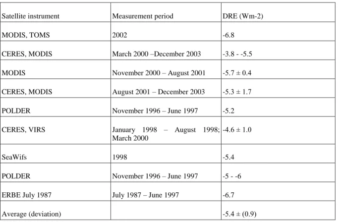
Table 2.2 summarises the most important parameters of satellite instruments which could be applied in determination of optical characteristics. The direct effect of aerosols can be characterised by three different parameters: (i) The optical thickness of aerosol, , indicates the ratio of the Sun radiation which does not reach the surface: Using this parameter as a negative exponent of the e ―natural number‖, we get this ratio. (ii) The albedo of a given aerosol layer shows the ratio of radiation reflected back towards the space in the given wavelength. (This term does not consider that part of the energy which is reflected from the surface.) Finally, (iii) the DRE, the common effect of natural and anthropogenic aerosols, indicates the surplus of outgoing energy from the Earth-atmosphere system compared to the situation without aerosols, at all.
The satellite based estimation concerning the direct effect of anthropogenic and natural aerosols on the short wave energy balance of the Earth-atmosphere system DRE influence is shown in Table 2.2. The different methods have given more or less the same value for the natural and anthropogenic direct radiation effect. The nine instruments using much more different approximation gave for this effect a -5.4 Wm-2 value. Comparing these values with the numbers of Fig. 2.2 we can express that their role is secondary beside the effect of cloudiness, atmospheric water content, or natural atmospheric greenhouse effect. On the other hand if we compare the latter effect (supposing that the natural and anthropogenic factors have got the same magnitude in DRE) with the magnitude of change the role of aerosol particles is not negligible either.
Table 2.2: Direct radiation effect by aerosols on the radiation balance of the Planet,estimated by satellite remote sensing (IPCC 2007: Table 2.3. abbreviated)
Satellite instrument Measurement period DRE (Wm-2)
MODIS, TOMS 2002 -6.8
CERES, MODIS March 2000 –December 2003 -3.8 - -5.5
MODIS November 2000 – August 2001 -5.7 ± 0.4
CERES, MODIS August 2001 – December 2003 -5.3 ± 1.7
POLDER November 1996 – June 1997 -5.2
CERES, VIRS January 1998 – August 1998;
March 2000
-4.6 ± 1.0
SeaWifs 1998 -5.4
POLDER November 1996 – June 1997 -5 - -6
ERBE July 1987 July 1987 – June 1997 -6.7
Average (deviation) -5.4 ± (0.9)
11. 2.4. Effects of land use
One of the poorly reconstructed anthropogenic influences on climate is the historical land cover change. Surface albedo, evapotranspiration and aero-dynamical roughness of an area could be affected in consequence of land use changes. The surface albedo modifies the short wave radiation budget. The surface roughness length modifies the efficiency of vertical exchange between the surface and the atmosphere in the planetary boundary layer.
Through the plant-specific rate of evapotranspiration to the potential one (the latter presumes unlimited water availability from the soil), the vegetation controls the partitioning of vertical turbulent heat fluxes between their sensible and latent forms. This proportion, in turn, influences the near-surface values of temperature and atmospheric humidity.
It is well known that climate is the main factor of vegetation development through the precipitation, temperature, radiation and through the carbon-dioxide content. But the vegetation changes also affect the climate (partly, but not only, as a feedback mechanism) via albedo, heat- water- and momentum fluxes, as direct effects on the energy balance. Besides that an indirect effect should also be considered which is based on changes in the CO2 concentration caused by the vegetation changes.
If all forests of the Earth were in their natural potential conditions, than their common area was 52-59 million km2. But the mankind uses substantial part of its continental surface for agricultural production and other effects (deforestation, urbanization, overgrazing, etc.). According to Crutzen (2002), on ca. 50 % of the continental areas natural surfaces are already changed by the mankind. Though this process started as early as with the occurrence of the stable climate conditions ca. 10000 BP, about 75 % of all forest reduction took place after the Industrial revolution.
One of the most significant changes in land use is the clearing of tropical forest in order to obtain new fertile areas for the agriculture, e.g. in the Amazon basin (Bonan, 2004). Though pastures of the tropical belt exhibit higher albedo than the forests, it was still computed that some warming is the net result of the forest reduction.
Further model simulation targeted the effect of land use changes on precipitation in the same region (Pielke et al., 1997). In the experiment there were differences in the land use parameters only with all atmospheric initial and boundary conditions retained unchanged. In case of natural vegetation the same weather situation could lead to intense convective cloudiness, but without precipitation. The same atmospheric conditions with the present agricultural land use could lead to intense precipitation and thunderstorm activity, as well. In the given period of time, the real observations supported the latter case with vast precipitation.
In arid and semi-arid regions of our planet the agricultural land use, the overgrazing and the use of trees for burning is able to modify the energy-balance of the surface, the hydrological cycle and, hence, the climate conditions, as well. The overgrazing increases the surface albedo, which, in turn decreases the temperature and vertical instability, hence the less convective cloudiness may lead to decreased precipitation in the given belts.
Hence, degradation of the landscape can even enhance the permanent drought. The more recent studies did also support, that large-scale changes of the land use of the Sahel-belt could lead to precipitation decrease even in the North-African regions (Clark et al., 2001).
Climate forming role of vegetation can even be seen in the transition zone between the tundra and taiga vegetations (Bonan, 2004). Differences in the albedo of taiga and tundra ecosystems, which are strongly driven by the lack or the existence of snow, can be an important regulating factor even at the larger scales for the atmospheric circulation. The taiga warms climate in contrast with the neighbouring tundra vegetation as it was found in several studies (e.g. Beringer et al., 2005).
Considering global effects of these changes, based on the land use data base by Ramankutty és Foley (1998), the strongest modifications took place in the last 300 years of forest degradation (mainly substituted by agricultural land use). In the previous 700 years (between ca. 1000 and 1700 AD) there is no significant effect of the land use changes in the global mean temperature. In the latter 300 years they are -0.09 °C in global mean and -0.15
°C in the Northern Hemisphere (Shi et al., 2007). At the temperate and high latitudes this effect was as high as - 0.3 °C with no considerable changes in the tropical and Polar regions.
Further studies supported the small decreasing effect of the land use changes on temperature, as well. But these studies did not consider the indirect effect through rising of the CO2 content of the atmosphere. This could, however, change the sign of the land use induced temperature changes from cooling to warming!
According to the estimations, 156 GtC was emitted into the atmosphere between 1850 and 2000 due to deforestation (Houghton, 2003). Brovkin et al. (2004) found that the land use was responsible for 15-35 % of the anthropogenic CO2 –emission depending on the details of the reconstructions according to Houghton (2003).
This means, the land use changes are among the attributed cases of the CO2- induced global warming, as well.
As fossil fuel burning increased rather fast in the recent century, the relative contribution of the land use to the atmospheric CO2 uptake decreased (Betts, 2006). Between 1850 and 1900 this value fluctuated between 42 and 68%, but in the 1990‘s this contribution was only 5-35 %. According to Matthews et al. (2004), the common direct and indirect effect of the land use changes could cause ca. +0.15 °C global in the 1700-2000 period. The global radiative effect of land cover change on climate was also estimated by Hansen et al (1998) and further reports were also published by the recent two IPCC Reports (2001, 2007), as well.
12. 2.5 Greenhouse gases and other problems of air chemistry
One may think that climate change and greenhouse gases are so often mentioned even in the public media that it may be a key to other problems of the environment, as well. But, as we can see below, this is not the case!
Fig. 2.5 indicates the five most important problems of atmospheric chemistry. They are the acid rain, the summer smog (high ozone), the ozone-hole (low ozone), the enhanced aerosol concentrations and the greenhouse effect, together represent ca 25 different chemical formations. None of them are involved in more than 3 problems. This means that a reduction of them does not solve all problems at once, though it is often hypothesized by laypersons.
One should tackle all these problems of the environment and their primary causes, the emission of the various atmospheric constituents, separately!
Figure 2.5: Five important problems of the atmospheric chemistry, indicating the key chemical components that play a key role in the selected issues. No one component influences more than 3 problems!
3. Climate change detection and attribution
13. 3.1 Attribution of the changes
Changes of climate can always be traced during the earth's history. For example, paleoclimates show a series of quasi-periodic variations and glacial periods returning at about 100 000-year intervals throughout the Quaternary era. These variations have been related to changes in orbital parameters causing changes in the solar radiation balance of the Earth. Typical examples are the processes of repeated glaciations in the Quaternary, the period of the "Climatic Optimum", 5-6 thousands years ago that was warmer and more humid than climate of present, or the "Little Ice Age", that lasted for a few hundred years and ended about 1850.
Historical changes have two common features: they were relatively slow and the processes were of natural origin in every case. In the recent century the situation has very likely been changing. Besides the natural forces, human activity has been added to the climate determining factors. In a few decades it can bring about changes of the present climate of such extent and rate that has not been experienced in the past one hundred thousand years.
There is a broad agreement among the scientific reconstructions of mean air temperatures over the Northern Hemisphere. All series show similar long term trends: warming from the start of the century to around 1940, cooling to the mid- 1960-s and early 1970-s, and continuous warming thereafter. However, the key question of the issue is if really the mankind is the responsible for the experienced global warming.
Fig. 3.1 shows us the strongest argument for this statement, at least in the last 50 years. The observed series of the global mean temperature are successfully simulated by the interval of 14 global climate models reproducing the past changes under the influence of all known anthropogenic and natural climate forcing factors. But, if leaving out the anthropogenic ones, i.e. allowing just natural factors, like volcanic eruptions and solar activity to act, this kind of simulation clearly departs from the fact. So, the warming of the recent half century could not happen without the anthropogenic factors. This statement can be erroneous in case of two parallel strong mistakes, only. The first error, in case, would be that scientist strongly overestimates the effects of greenhouse gases in their computations, whereas the second one is that the ―true‖ reasons of the observed warming, are not known, at all. Probability of these two mistakes is assessed by the IPCC WG-I, (2007) as ≤ 10 %. Until this unlikely combination becomes proven, the only smart decision is to get prepared to further warming, as it follows from the ≥ 90 % likelihood of the anthropogenic origin.
Figure 3.1: Comparison of observed continental- and global-scale changes in surface temperature with results simulated by climate models using natural and anthropogenic forcings. Decadal averages of observations are shown for the period 1906–2005 (black line) plotted against the centre of the decade and relative to the corresponding average for 1901–1950. Lines are dashed where spatial coverage is less than 50%. Blue shaded bands show the 5–95% range for 19 simulations from 5 climate models using only the natural forcings due to solar activity and volcanoes. Red shaded bands show the 5–95% range for 58 simulations by 14 climate models using both natural and anthropogenic factors. {IPCC, 2007: FAQ 9.2, Figure 1}
One may think that due to the technical problems of near-surface temperature observations, already mentioned in Chapter 2, the trends of this value may be uncertain. In idea it is so, but a rather convincing fact is that in four different analysis centres, possessing historically differing sets of data from all over the world, the analysed trends are rather similar (Fig. 3.2). From this we can also see that the globally warmest years were 1998, 2005 and 2010, with small differences among each other compared to the estimation error (ca. 0.03 K).
Figure 3.2: Global mean temperature as reconstructed by four international data centres: NASA Goddard Institute for Space Studies, NOAA National Climate Data Centre, Meteorological Office Hadley Centre/Climate Research Unit and the Japanese Meteorological Agency. Credit: NASA Earth Observatory/Robert Simmon.
14. 3.2 Comparison with the last 1000 years
The last 100 years is a smaller segment of time with very likely anthropogenic influence along its path. This 20th century's temperature trend is antecedent to the one for the ca. 900 previous years (Fig. 3.3). This is also much faster with its ca. 0.7-0.8 K/century pace than the previous ca. -0.3 K/millennium cooling. (The sources of
the reconstructions are seen on the figures at the cited source
(http://www.ipcc.ch/publications_and_data/ar4/wg1/en/ch6s6-6.html#6-6-1).
Figure 3.3: The reconstructed annual mean temperature (K) of the northern hemisphere compared to the average of the 1961-1990 reference period. (Source: IPCC 2007, Fig. 6.10)
Though, we have mach less information on the external forcing factors during the whole millennium, several climate modellers tried to reconstruct the global mean temperature along this long period, as well (Fig. 3.4). The attempts are fairly successful: the long-term trend and the majority of the inter-decadal fluctuations are more or less caught by the simulations.
Figure 3.4: Reconstructed mean temperature of the northern hemisphere (K) as compared to the 1961-1990 period. (Source: IPCC 2007, Fig. 6.13d)
This is important, since it means there were no unknown turns in climate of the Earth. Hence, one may hope that such surprises will not happen even in the future. In other reading: There is a very little chance that warming of the recent century was caused by natural factors.
15. 3.3 Capability and limitations of the present climate models
At present, General Circulation Models (GCMs) are the only climatic models, that are useful for regional considerations. GCMs develop in two directions, utilising the possibilities of the super-computers. Global Atmospheric GCMs (AGCMs) have nominal (grid-point distances or equivalents in terms of truncation) resolutions of 100 - 200 km.