Soil & Tillage Research 209 (2021) 104959
Available online 17 February 2021
0167-1987/© 2021 The Author(s). Published by Elsevier B.V. This is an open access article under the CC BY-NC-ND license
(http://creativecommons.org/licenses/by-nc-nd/4.0/).
Long-term effects of conservation tillage on soil erosion in Central Europe:
A random forest-based approach
Bal ´ azs Madar ´ asz
a,b,*, Gergely Jakab
a,c, Zolt ´ an Szalai
a,c, Katalin Juhos
b, Zsolt Kotrocz ´ o
b, Adrienn T ´ oth
a, M ´ arta Lad ´ anyi
daGeographical Institute, Research Centre for Astronomy and Earth Sciences, Buda¨orsi út 45, 1112 Budapest, Hungary
bDepartment of Agro-Environmental Studies, Institute of Environmental Science, Szent Istvan University, Vill´ ´anyi út 29–43, 1118 Budapest, Hungary
cDepartment of Environmental and Landscape Geography, Faculty of Science, E¨otv¨os University, P´azm´any P. 1/C, 1117 Budapest, Hungary
dDepartment of Biometrics and Agricultural Informatics, Institute of Mathematics and Basic Sciences, Szent Istv´an University, Vill´anyi út 29–43, 1118 Budapest, Hungary
A R T I C L E I N F O Keywords:
Runoff Soil loss Modelling SOM WSA Earthworms
A B S T R A C T
Conservation tillage (CT) is of primary importance in food security, soil conservation, and sustainable devel- opment, even though its comprehensive effects on runoff (RO) and soil loss (SL) are still not fully understood. In 2004, a field-scale study was launched in southwest Hungary to investigate the long-term (16 years) effects of CT on RO, SL and soil, under a warm-summer humid continental climate. Four, especially large, 1200 m2 plots (2 ploughing tillage (PT) and 2 CT) were established, using a special, two-channel collection system. By the end of the study period, significantly higher water-stable aggregates (PT: 20.0 %, CT: 30.4 %), higher soil organic matter (PT: 1.4 %, CT: 1.9 %), greater earthworm abundance (4.9 times that in PT plots) was recorded on the CT plots. Conservation tillage decreased surface RO by 75 % and SL by 95 %. The difference between PT and CT was significant for mean annual soil erosion, with values of 2.8 t ha−1 and 0.2 t ha-1, respectively. The exceedance of extreme precipitation events was <2%, but their impact on soil erosion was extraordinarily high. Runoff and SL were predicted for the whole dataset, and for the sub-dataset of maize culture, in four separate Random Forest (RF) model developments. The often used linear models are not suitable for predicting soil erosion, hence a more robust, non-parametric, advanced method of classification tree analysis was used. The RF classification method was able to predict erosion risk. For the maize sub-dataset, the RF model best predicted the extreme events, followed by the no-runoff category. The sensitivity of the groups with the highest and lowest risk all exceeded 82
% for SL and 64 % for RO. Tillage type was the most important factor. This long-term study demonstrated that the use of CT enabled the maintenance of a major fraction of precipitation on arable land, and consequently, soil loss remained an order of magnitude lower than its tolerable value. The RF method is suitable for modelling RO and SL. In future, the integration of more datasets in modelling would considerably improve the precision and accuracy of prediction of RO and SL.
1. Introduction
The study of agriculture is an ancient topic. The ambitions of increasing soil fertility, preventing its decline and avoidance of oscilla- tions of yields date back to the dawn of agriculture (Zeder, 2011). Soil is one of the most important natural resources; its protection is of major importance. In Europe, 12 % of soils are exposed to soil degradation due to intensive agriculture and are affected by severe water erosion (Oldeman et al., 1991). Soil loss (SL) (17 Mg ha−1) greatly exceeds the
rate of soil formation (1 Mg ha−1) (Troeh and Thompson, 1993), which is therefore the maximum tolerable SL. In Hungary, over one-third of croplands are eroded (2.3 million ha; Kert´esz and Centeri, 2006). To overcome this problem, several erosion mitigation techniques have been introduced worldwide and new tillage systems are becoming wide- spread (Kassam et al., 2017, 2019). Today, conservation agriculture is one of the most modern agricultural systems. This sustainable, cost-efficient, and water-saving management system may offer future prospects because beyond soil erosion mitigation, it also improves food
* Corresponding author at: Geographical Institute, Research Centre for Astronomy and Earth Sciences, Budaorsi út 45, 1112 Budapest, Hungary. ¨ E-mail address: madarasz.balazs@csfk.org (B. Madar´asz).
Contents lists available at ScienceDirect
Soil & Tillage Research
journal homepage: www.elsevier.com/locate/still
https://doi.org/10.1016/j.still.2021.104959
Received 31 August 2020; Received in revised form 27 January 2021; Accepted 28 January 2021
security and reduces resource degradation even under weather anoma- lies such as drought and intense rainfall events (Holland, 2004; Derpsch et al., 2010; Busari et al., 2015). Conservation tillage (CT) is one of the most widespread tillage systems that define conservation agriculture.
In contrast to conventional ploughing tillage (PT), CT is a non- inversion tillage system, where at least 30 % of crop residues remain on the surface; CT reduces the number of wheel paths and minimises soil disturbance (by omitting tillage steps and by the application of com- bined machines). Several variations of CT are practised, depending on the depth and width of the tillage, including no-till, ridge-till, strip-till, mulch-till, and reduced-till. The diverse forms of CT are applied to approximately 200 Mha worldwide (Kassam et al., 2019). In Europe, it was practised on 22.7 Mha in 2010, or 26 % of arable lands (Kert´esz and Madarasz, 2014). ´
A number of studies have been dedicated to examine the benefits of no-till (Blevins et al., 1983; Six et al., 2002; Okada et al., 2014; Merten et al., 2015; Gao et al., 2019), but little research has been published on impacts on soil erosion of reduced-till, a simpler, and somewhat less innovative, but more widespread, practice. In Hungary, no-till is applied to less than 1% of arable land. The proportion of the other CT technol- ogies, most of which can be regarded as reduced-tillage, is slowly increasing and was slightly over 11 % in 2010 (Kert´esz and Madar´asz, 2014).
Conservation tillage is considered an effective way of increasing water infiltration and reducing runoff (RO) and soil erosion. Conserva- tion tillage can reduce RO by ~50 %–70 % and SL by ~70 %–95 %, depending on the type of CT applied, and other environmental condi- tions, including climate, slope, and plant cover (Strauss et al., 2003;
Raczkowski et al., 2009; Xiong et al., 2018; Zhao et al., 2019).
The reduction of SL may be the result of the interaction of several factors (for example, increased aggregate stability, infiltration and humus content, limited crusting, vegetation cover, and tillage; Cheng et al., 2018). Almost all of these are related to soil structure, function and biological activity. One of the greatest advantages of CT is that it does not damage the layer-specific structure of soil activity. This intact structure, together with the crop residues in the near-surface zone, in- creases the humus content of the soil, improve soil structure, and in- crease the formation of water-stable aggregates. Experimental studies have confirmed that CT has a beneficial influence on the activity of earthworms compared to PT (Birk´as et al., 2004; Rothwell et al., 2005;
Eriksen-Hamel et al., 2009; Dekemati et al., 2019). The biological ac- tivities of earthworms create stable gallery networks, which form a system of macropores capable of increasing rates of infiltration of sur- face water and improving soil aeration.
During the past few years, an increasing number of long-term tillage studies have been undertaken in widely separated climatic regions, providing robust results, compared to earlier short-term (a few-years) studies. Previous studies have examined the efficacy of CT systems from diverse perspectives, including yield (Grigoras et al., 2011;
Madarasz et al., 2016; Kurothe et al., 2014; Dekemati et al., 2019), soil ´ erosion and the role of soil organic carbon (Six et al., 1999; Rhoton et al., 2002; Melero et al., 2009a, 2009b; Jakab et al., 2019; Van den Putte et al., 2012).
In addition to the long-term analysis, the size of the plots is also a key factor in the study of soil erosion (Leys et al., 2010). The interpretation of soil erosion measurements is entirely a problem of scale (Chaplot and Poesen, 2012): up- and downscaling the results are very site-specific processes; thus, their use for general modelling is limited (Stroos- nijder, 2006; Leys et al., 2010). There are a large number of papers reporting and interpreting data pertaining to RO and SL, especially at a plot-scale, but a significant need for additional erosion studies remain, particularly to fill in the gaps in less-studied fields/sizes (Poesen, 2015).
Field-scale and long-term plot measurements, including large-scale op- erations, for example tillage and plant protection, remain important.
The number of long-term, field-scale experiments is very limited in the continental sub-humid region of Europe (Prasuhn, 2012). Klik and
Rosner (2020) investigated the effects of no-tillage (NT) and mulch-tillage (MT) on soil erosion, from spring to autumn, in Austria.
They used plots of 240–480 m2. Prasuhn (2012) did not use plots for erosion measurements and used 203 crop fields to estimate the effect of tillage on soil erosion, over 10 years, in the Swiss Midlands. His results suggested that SL was more than an order of magnitude lower under NT and MT than under PT. In several cases, soil erosion due to changes in tillage practise has been studied in an area of only a few 100 m2 (Zhang et al., 2015; Tuan et al., 2014; Gao et al., 2019). In other cases, rainfall simulation experiments were conducted across even smaller areas (a few m2) and these results are hardly interpretable at a field- or catchment-scale (Kinnell, 2016).
The main purpose of soil erosion measurements is to understand and predict the process itself. One critical step is to identify key factors closely related to SL and erosion risks. The traditional approach for the selection of essential variables is a regression (Wu et al., 2018; Klik and Rosner, 2020) and general linear models (Francke et al., 2008). This approach requires the assumptions that predictor variables have a linear relationship with the dependent variable, and the model residuals are normally distributed. However, such relationships are rarely linear, and normality is frequently highly violated, given the frequent extreme erosion events and the skewed distribution in the data. In such cases, linear models are not suitable for predicting soil erosion (Klik and Rosner, 2020).
Statistical modelling, based on machine-learning algorithms, can provide alternatives to traditional linear approaches and overcome some of their limitations (Chaudhary et al., 2016). For example, classification and regression trees (CARTs) can predict continuous or discrete dependent variables (e.g., RO and SL) using continuous or discrete predictor variables (e.g., soil parameters, slope, precipitation, vegeta- tion cover) (de Graffenried and Shepherd, 2009; Gayen and Pour- ghasemi, 2019). The purpose of the analyses via tree-building algorithms is to determine a set of if-then logical conditions that permit accurate prediction or classification of cases. Random Forests (RF) is a more robust, non-parametric, advanced method of classification tree analysis that can also predict erosion (Francke et al., 2008; Zimmermann et al., 2012; Mohr et al., 2013; Cheng et al., 2018). Databases from long-term field-scale experiments, on which mathematical modelling can be performed, are therefore of great importance.
In this study, the long-term effects of CT and PT on RO, SL, and soil, under arable cropping, were analysed under continental, sub-humid conditions of Central Europe. The results of 16 years (2004–2019) of precipitation, RO, and SL monitoring at a field-scale experimental site were evaluated. We examined long-term changes in soil quality as a result of the change in tillage. Furthermore, we investigated the possi- bilities of modelling RO and SL using tillage, precipitation, and vege- tation cover data. We predicted RO and SL for the whole data set and the sub-dataset of maize culture in four separate Random Forest model developments.
2. Material and methods
2.1. Site description
The study area is located in southwest Hungary, in a hilly region 7.5 km west of Lake Balaton, near the village of Szentgy¨orgyv´ar (46.748 ◦N, 17.147 ◦E, 150 m a.s.l.) The climate is warm-summer humid continental (K¨oppen, 1936). Long-term mean annual temperature is 11 ◦C and mean annual precipitation is 700 mm (Haj´osy et al., 1975). During the study period, between 2004 and 2019, mean annual temperature was similar to the long-term record, but mean annual precipitation was only 628 mm (438–870 mm) (Fig. 1). The slope of the field-scale experimental site was 10 %. The parent material is loess and the soil is eroded silty loam Luvisol with low soil organic matter content (WRB, 2014). The study site was previously conventionally tilled for decades and basic soil proper- ties were analysed before the establishment of the experimental plots in
2003 (Table 1).
2.2. Experimental design and tillage systems
The experiment was initiated in 2003 as part of the SOWAP (Soil and Surface Water Protection Using Conservation Tillage in Northern and Central Europe) project to study PT and CT in a comparative manner (Field et al., 2007; Kert´esz et al., 2007; Lane, 2007; B´adonyi et al., 2008a, 2008b; Madar´asz et al., 2011). For the erosion experiment of PT and CT, 2 ×2 identical plots of 24 ×50 m (width ×length, 1200 m2) were established. Plots were isolated from the rest of the slope using metal bunds. Agricultural tillage is still possible on plots of this size, but their size is small enough for the proper collection and measurement of RO and SL. The order of the plots was PT1, CT1, CT2, and PT2. The only difference between the plot pairs was the tillage type; they received the same treatment in every other aspect (crop rotation and crop type, fer- tilisation, weed control, and plant protection).
Cultivation of the plots was across-slope. The PT consisted of mouldboard ploughing (to 25–30 cm depth), harrowing, and seed-bed preparation every year. The CT was a plough-less, non-inversion tillage operation, which was characterised by a reduction in the number of tillage operations, leaving ~30 % of the soil surface covered with crop residues. During the first three years, CT consisted of shallow discing (8–10 cm), but later, due to continual weed problems, a cultivator was applied (8–10 cm). In addition, in three years (2007, 2012, and 2015), medium deep (20–25 cm) subsoiling was undertaken across the entire study area. During the 16 years of the research, maize (8 times), winter wheat (3×), oilseed rape (2×), sunflower (2×), and spring barley (1×) were produced in crop rotation. Four cover crops were included in the rotation in all plots (2015–2018).
Yield data were collected from each plot; however, the 0.12 ha area plots provided limited capacity for a precise comparison. Therefore, yields were studied on 10 plot-pairs, with an area of 105 ha, on a nearby experimental site. For the description and methodology of this research, refer to Madar´asz et al. (2016).
2.3. Sampling and measurements
A special, two-channel collection system was developed for the measurement of RO in a way that enabled collection of RO of both the frequent, low-intensity events and the rare (<1% probability), high- intensity, precipitation events. In this system, the RO was led into
three 1 m3 collecting tanks (with 0.8 m3 useful volume) with 1/9 divi- sion between them, resulting in a total (0.8+[9 ×0.8]+[9 ×9 ×0.8]) 72.8 m3 capacity. A detailed description of the measuring system is given by Kert´esz et al. (2007). After each RO event, RO was stored to allow sedimentation for one day, and the volume of the liquid portion was then determined, and the sediment soil was also measured and sampled. The sediment content of the oven-dried water and sediment samples was measured and used to calculate the SL and sediment con- centration of the RO. Meteorological data were collected by an auto- mated meteorological station at the experimental site every 5 min.
Runoff and SL data were clustered by the year of study as a factor, using the P´alfai Drought Index (PAI; P´alfai, 1988), which was developed specifically for climate conditions in Hungary, and expresses the importance of the distribution of precipitation throughout the growing season. The higher the index, the deeper the drought (PAI < 4 no drought, PAI 4–6 slight drought, PAI >6 moderate drought):
PAI= [∑Aug
i=Apr Ti
]
5 ∗100
10+Sept∑
i=Oct
(Pi∗wi)
(1)
where Ti is mean monthly temperature (◦C), Pi is monthly precipitation (mm), and wi is a weight constant.
In the spring of 2019, 18 soil samples (0–15 cm depth) were collected per treatment (9/plot) and used for determination of total organic car- bon (TOC) and microbial biomass carbon (MBC). All samples were composites of seven subsamples collected from a circle with a diameter of 1 m. Soil samples were air-dried for TOC, passed through a 2 mm sieve, and visible plant litter was removed. The TOC content was determined by dry combustion at 900 ◦C using a Shimadzu TOC-L device equipped with an SSM 5000A Solid Sample Combustion Unit (Jakab et al., 2016, 2019). The measured values were converted to soil organic matter (SOM) by multiplying by 1.72 (van Bemmelen, 1890).
After soil sampling, all samples were stored at 4 ◦C for MBC deter- mination. Microbial biomass carbon content was determined by the chloroform fumigation-extraction method (Vance et al., 1987; Paul et al., 1999) that killed most soil organisms by destroying their mem- branes and cell walls. The organic carbon (C) content of both the fumigated and non-fumigated samples was extracted by potassium sul- phate extraction, and the C content of the samples was determined using a Shimadzu TOC-L device equipped with an OCT-L Liquid Sample Unit.
Fig. 1.Annual precipitation and temperature at the erosion experimental site at Szentgy¨orgyv´ar (2004-2019). Data from the local automatic weather station.
Table 1
Physical and chemical properties of the 0–45 cm layers of soil profile representative for the experimental field in 2003 (n =6). SOM: Soil Organic Matter; Clay =<2 μm; Silt =2–20 μm; Sand =20–2000 μm.
Depth pH (H2O) pH (KCl) SOM CaCO3 Bulk density Clay Silt Sand
cm – – % % g cm−3 % % %
0–15 6.25 4.80 2.31 0.00 1.37 3.94 59.63 36.43
15–30 6.28 4.57 2.08 0.00 1.57 3.68 57.20 39.12
30–45 6.36 4.72 0.45 0.00 1.59 4.80 58.46 36.74
The C content of MBC was determined as the difference between the C content of non-fumigated and fumigated samples, from which biomass was calculated, according to Vance et al. (1987).
The number and weight of earthworms were determined as in- dicators of biological activity. Earthworm sampling was conducted 9 times during the first 5 years of the experiment (2002–2008) and 6 times during the last four years (2016–2019) of the research. If weather and soil conditions enabled sample collection, samples were collected in spring and autumn, according to the method described by Harper Adams University College (2003). Samples were taken at 9 points on each plot using a cylinder 10 cm in diameter and height. Earthworms were selected and weighed manually from the soil samples.
The ratio of water-stable aggregates (WSA) was measured in the spring of 2017. Nine samples were collected from the surface (0–10 cm) of each plot, with 18 samples per tillage type. The 1–2 mm grain size fraction was sieved from air-dried samples (Retsch AS200). Aggregate stability was then examined using the Eijkelkamp wet sieving apparatus by determining the ratio of soil aggregates >250 μm (Kemper and Koch, 1966). Soil aggregates were disintegrated using 0.1 M Na-pyrophosphate and the remaining sand fraction >0.25 mm was sieved and weighed. The percentage of stable aggregate fraction was calculated by subtracting the weight of the sand fraction from the total weight of the 0.25–2 mm grain size fraction (Villar et al., 2004).
2.4. Testing the effect of tillage on runoff and soil loss
Statistical analysis was undertaken using R 4.0.0 (R Core Team, 2020). To normalise the variables, RO and SL were transformed by ln (x+0.001) to ensure that the absolute values of skewness and kurtosis were both below 1.5 (n =560). Pearson’s correlation of the transformed variables was highly significant (PT: R2 =0.65, p <0.001; CT: R2 = 0.64, p <0.001). The RO and SL, as dependent variables, were evaluated using a four-way multivariate analysis of variance (MANOVA), with factors tillage, crop, year, and month. The normality of residuals was checked again by the absolute values of their skewness and kurtosis;
they were all below 1. Homogeneity of variances was accepted for tillage levels because the ratios of maximum and minimum variances were both below 2. However, the assumption of homogeneity of variances was slightly violated for the factor crop (the ratios of the maximum and minimum variances were 2.4 and 1.9 for RO and SL, respectively). We calculated the Wilk’s λ and performed a follow-up four-way ANOVA with Bonferroni’s correction, for both dependent variables, to detect the tillage effect. Finally, Games-Howell’s post hoc test was undertaken to separate the homogeneous subsets. The effect of PT and CT treatments were compared for variables SOM, WSA, and ln(MBC) by Student’s t test (their normality was accepted because the absolute values of their skewness and kurtosis were below 1 and their variances were homoge- neous, as demonstrated by the F test, with p >0.05); for the number of earthworms by Fisher’s exact test; for the weights of earthworms, by two-way ANOVA with factors treatment and time (assumptions were
proven by skewness, kurtosis, and Levene’s test); for ln (annual RO + 0.001), ln(annual SL +0.001), and the number of yearly runoff events, by one-way MANOVA (assumptions were also tested and satisfied); for the precipitation events ratios by Z test; for the sediment concentrations, by two-way ANOVA with factor treatment and whether the RO event was above or below 1 mm; and for sediment concentration of maize plots, by Student’s t test (assumptions were proven by skewness, kur- tosis, and Levene’s or F test).
The exceedance (E; [%]) is the percentage of RO/SL events that exceed a given amount of RO/SL. It is calculated by a non-parametric method, where the observed events are ordered in terms of their size, and numbered from the largest to the smallest (m), the total number of events (N) is considered.
E =100* m / (N +1) (2)
2.5. Random Forest modelling
Our long-term dataset (2004–2019) consisted of 560 records of 140 RO events and associated precipitation, RO, and SL data. One RO event is a precipitation event leading to RO that occurs with at least a 6 h gap between previous and subsequent events. Four factor - and three numeric-type predictor variables (features) were selected: crop culture (the majority was maize with 244 records, wheat, sunflower, rape, spring barley, no-crop/stubble), tillage (PT and CT), plant cover (1–5 from 0 to 100 % by 20 %), the month of the event, precipitation amount (mm), precipitation duration (h), precipitation intensity (maximum in- tensity of 30 min, I30, mm h−1 by Wischmeier and Smith, 1978). Plant cover was determined monthly, by visual survey, on 1 m2 with the help of a 1.0 ×1.0 m frame, with 5 replicates. Runoff and SL served as the two dependent variables, both divided into four categories because the database was not suitable for regression analysis. During the 16 years of the experiment, electrical and equipment failures, animal damage, and lightning hit the meteorological station. Consequently, approximately 20 % of precipitation data are missing. The RO and SL categories, together with the total number of missing precipitation data, are pre- sented in Table 2.
Model development was conducted in R 4.0.0 (R Core Team, 2020) with packages ‘randomForest’ (Liaw and Wiener, 2002; Breiman et al., 2006.), ‘caTools’ (Tuszynski, 2020), ‘e1071’ (Meyer et al., 2019),’ caret’
(Kuhn, 2020) ‘vcd’ (Meyer et al., 2020) and ‘gdata’ (Warnes et al., 2017) to perform Random Forest (RF) models. Figures were produced using the package’ ggplot2’ (Wickham, 2016). Random Forest is a multivariate, nonparametric algorithm based on the Classification and Regression Tree (CART) that handles missing data of independent variables well (Breiman, 2001). We aimed to predict dependent variables RO and SL for the whole data set and for the sub-dataset of maize culture in four separate RF developments. With RF, we could manage missing values issues very successfully by imputing those using proximities (Tang and Table 2
The rates of runoff (RO) and soil loss (SL) classified into four categories with total number of RO and SL records (Total), the total number of RO and SL records with maize culture (Total maize) and the total number of missing values from the feature variables precipitation amount, precipitation duration and precipitation intensity (Missing and Missing maize).
Categories Group Total Missing Total maize Missing maize
Runoff (RO, mm)
RO=0 1 245 55 69 3
0 <RO<=0.3 2 203 59 95 21
0.3 <RO<1.2 3 52 10 34 4
1.2 <=RO 4 60 8 46 4
sum 560 132 244 32
Soil loss (SL, t ha−1)
SL=0 1 181 39 45 2
0 <SL<=0.03 2 193 59 92 17
0.03 <SL<0.15 3 97 23 49 8
0.15 <=SL 4 89 11 58 5
sum 560 132 244 32
Ishwaran, 2017).
We split the dataset into training and test subsets randomly at a fixed rate (75 % and 25 %). Random Forest works with a high number (ntree, default =500) of datasets from the training data set created by random sampling with replacement (bootstrapping) and develops a very large number of decision subtrees. The data set that is not used in a step (approximately 1/3) is called Out-Of-Bag (OOB). In each step, the al- gorithm uses not all predictor variables (features), just a fixed number of them (mtry, default ≈square root of the number of features), randomly.
The decision subtrees developed from the training dataset were used to identify a classification consensus by selecting the most common output.
This is then tested for the remaining test dataset.
To measure the classification quality of the RF model with respect to the test data set, we used the following measures: percent of records correctly classified (accuracy), true positive classification rate (sensi- tivity or recall S), true negative classification rate (specificity), balanced accuracy (average of sensitivity and specificity), positive prediction value (precision, P), negative prediction value, prevalence, detection rate, detection prevalence (Tharwat, 2018), and the area under the receiver operating character (ROC) curve (AUC; Fawcett, 2006; Hosmer and Lemeshow, 2000), and the error rate of the tree if it is applied to the OOB data (OOB error), and the F1 score defined as:
F1=2∗P∗S
P+S (3)
based on Powers (2011).
We optimised the RF parameters mtry and ntree with respect to the OOB error estimate and root mean square error (RMSE), considering other classification quality measurements, such as accuracy, F1 score, and AUC, and finally set them to ntree =400, 500, or 550 and mtry =4 or 5. As a splitting rule, we applied the mean decrease in accuracy and
the mean decrease in the Gini Index (Strobl et al., 2006). We calculated the variable importance based on the overall mean decrease in accuracy (MDA) and categories (Strobl et al., 2008; Louppe et al., 2013; Gregor- utti et al., 2015). For this, we used the OOB sample set to calculate ac- curacy. The values of a specific feature were then randomly shuffled, while all other feature values remained the same and the accuracy of the shuffled data was calculated. Finally, we took the difference between these two accuracy values and their mean across all trees (MDA). This importance measure is the overall MDA, while breaking them down by outcome categories, and MDA can also be provided for each category.
The rate of agreement between observed and predicted classifica- tions can be measured by Cohen’s Kappa (Cohen, 1960). However, the rates of RO and SL, ranked from 1 to 4, range from no risk through medium, high and very high risk. Thus the misclassification cannot be treated equally when it is predicted, for example, no risk or high risk when the case is very high risk. Therefore, we preferred to use the weighted Kappa (Cohen, 1968), which assigns increasing weights to increasing misclassification errors, so that different levels of agreement can contribute to the value of Kappa (Fleiss and Cohen, 1973; 2003).
3. Results and discussion
3.1. Investigation of factors influencing runoff and soil erosion 3.1.1. Soil organic matter
Soil organic matter was significantly higher in the topsoil (0–15 cm) of CT than PT (t(34) =14.82, p <0.001). The low mean SOM content of PT (1.4 %) and 1.9 % of CT plots is similar to typical values of eroded Luvisols (Fig. 2A).
The 34 % higher value of SOM under CT resulted in a small rate of accumulation of annual soil organic carbon (SOC) (0.18 Mg C ha–1
Fig. 2. Distribution of soil organic matter (A), water stabile aggregates (B) and microbial biomass carbon (C) for the experimental plots at Szentgy¨orgyv´ar. PT:
Ploughing Tillage, CT: Conservation Tillage. Quality of soil structure is given by Bartlova et al. (2015).
year–1). The increase in SOM as a consequence of CT has been described in several studies, with values differing site-to-site (Angers et al., 1997;
Gonz´alez-S´anchez et al., 2012; Piazza et al., 2020). Piazza et al. (2020) reported a similar scale of increase in Italy. As a result of the plant residues remaining and tillage with no rotation, this increase is typically concentrated near the surface (L´opez-Fando and Pardo, 2011; G´al et al., 2007; Dekemati et al., 2019). The positive effect of CT can partly be explained by the large increase in SOC content in the topsoil, which improved the stability of soil aggregates (Rhoton et al., 2002).
3.1.2. Water stable aggregates
The average WSA value of PT was as low as 20.0 %. This was significantly higher under CT (30.4 %; t(34) =2.91, p <0.01; Fig. 2B).
This rate was only sufficient to reach the upper threshold of the low quality structure category (Bartolova et al., 2015). However, the 52 % higher mean WSA value under CT reflects an improved aggregate structure and stability, which can eventually increase water infiltration, consequently decreasing erodibility. Similar to PT, Li et al. (2019) observed a 55 % increase of the WSA in an area of no-till with residue retention. These significantly higher WSA values are characteristic of the uppermost 5 cm of soil that is most exposed to erosion. At 5–15 cm depth, only a moderate increase of WSA was observed previously (Karlen et al., 2013). The increase in SOM and WSA under CT is also in agreement with the results of Rhoton et al. (2002), who found a strong relationship between aggregate stability and SOM (R =0.92, p <0.01).
3.1.3. Earthworm investigations
In the spring of the first research year (2004), the ratio of earthworm abundance in CT to PT plots was 1.0 (21 in.. m−2). Across the entire time period, this ratio was 4.9, in accordance with the 2–9-fold increase observed previously (Chan, 2001; Dekemati et al., 2019); however, the standard deviation of the annual values was high. A significant differ- ence was observed between the tillage types during the first two years after the tillage shift (Fisher’s 2004–2005: F = 16.12, p < 0.001;
2018–2019: F =42.77, p <0.001). The comparison of data from the first and last two years (2004–2005 and 2018–2019) demonstrated an in- crease of the absolute number of earthworms in soil under both tillage types (CT: 3.1 times, F =43.54, p <0.001; PT: 4.5 times, F =21.62, p <
0.001; Fig. 3), probably due to the introduction of the cover crop in crop rotations during the last 4 years (Roarty et al., 2017). Although the in- crease was higher in PT plots, this means merely 55 earthworms m−2, while in CT 168 earthworms m−2 were recorded. Consequently, on average, 3–5 times more earthworms occurred. The larger earthworm activity under CT leads to an increase in the WSA and topsoil SOC, the formation of macropores at the surface, and stable gallery networks, which increase infiltration, and thus reduce RO and erosion (Ehlers, 1975). The average weight of the earthworms ranged between 0.1 and 0.5 g (Fig. 3B). The two-way ANOVA test demonstrated that both tillage treatment and time effects were significant (F(1;109) =4.58, p <0.05; F (1;109) =7.52, p <0.01, respectively). Earthworm weights under CT
were somewhat larger than the averages in the first and last two years, but the tillage effect was significant only in 2004–2005 (F(1;27) =4.38, p <0.05; 2018–2019: F(1;83) =2.08, p =0.15). The difference between years was significant for PT only (F(1;25) =8.40, p <0.05; CT: F(1;81)
=3.63, p =0.06). Six species of earthworm were distinguished in the study area (Aporrectodea caliginosa, Aporrectodea rosea, Allolobophora chlorotica, Octolasium lacteum, Lumbricus rubellus, Proctodrilus tuber- culatus), spending their active period within the upper 20 cm of the soil.
3.1.4. Microbial biomass carbon
Microbial biomass studies, contrary to our expectations, did not show a significant difference between the two tillage systems (t(27) = 0.07, p =0.94). The amount of MBC was 166.3 μg g−1 for PT and 129.4 μg g−1 for CT, with coefficients of variation (109.1 %, 76.1 %, respec- tively; Fig. 2C). Sampling took place in spring, when the low tempera- ture of the previous winter, combined with low soil moisture content, could be the reason for the lack of difference (Zelles et al., 1991; Fekete et al., 2016). Nunes et al. (2020).
3.2. Effects of treatment on runoff and soil loss
Mean annual RO from PT and CT plots was 18 mm and 4 mm, respectively, while mean SL was 2.8 t ha−1 and 0.2 t ha-1, respectively.
These differences were significant, as was the annual number of runoff events (Wilk’s λ =0.76, p =0.05; annual RO: F(1;30) =7.53, p <0.05;
Fig. 3. Mean number and weight of earthworms for the experimental plots at Szentgy¨orgyv´ar in the period of 2004–2005 and 2018–2019. PT: Ploughing Tillage, CT:
Conservation Tillage. Different letters represent significant differences (p <0.05). Upper case: Comparison of elapsed time effect under fixed tillage; Lower case:
comparison of tillage effect in a fixed year.
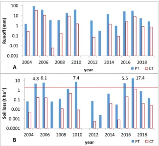
Fig. 4.Distributions of annual runoff (A) and soil loss (B) under PT (Ploughing Tillage) and CT (Conservation Tillage) treatments at Szentgy¨orgyv´ar (2004–2019). Red line: Soil loss tolerance value (2 t ha−1).
annual SL: F(1;30) =9.38, p <0.05; annual number of RO events: F (1;30) =6.70, p <0.05), respectively). Thus, RO was reduced by 75 % and SL by 95 %, from CT plots. The distributions of annual RO and SL between 2004 and 2019 are shown in Fig. 4.
The acceptable magnitude of SL is the topic of a longstanding debate (Holý, 1980; Bronger et al., 2000; Davis, 1982; Hall et al., 1985; Dazzi et al., 1998). In Hungary, the normative value of 2 t ha−1, published by Centeri and Pataki (2003), is considered to be the most relevant (Jakab et al., 2010). Soil loss from CT plots remained much lower than this value in each year, with a maximum value of only 1.3 t ha-1. A favour- able impression is suggested by the 16-year average of PT; however, examination of the yearly data revealed five major outliers. The largest annual rate of SL (17.4 t ha−1) was measured in 2017 under maize, which was 8.7 times larger than the rate of soil formation (Fig. 4B). Soil loss values are considered low for both tillage types, which is partly a consequence of the use of cross-slope cultivation (Quinton and Catt, 2004; Prasuhn, 2012).
Over the 16 years of study, 140 RO events were registered on PT plots (249 records), while there were only 78 on CT plots (130 records). Thus, during approximately half of all precipitation events that generated RO on the PT plots, no RO was generated from CT plots and all incoming rainwater infiltrated these plots. The standard deviation was large due to the large differences in monthly and annual precipitation. The lowest precipitation occurred in 2011 (438 mm) and no RO was recorded, despite maize growing on the plots. Conversely, in 2017, when maize was also sown, 18 RO events occurred (Fig. 4A). Klik and Rosner (2020) studied an area of similar slope and soil texture and reached similar conclusions.
The RO and/or SL values from the CT plots rarely exceeded those of the PT plots (6/140). In all cases, this occurred during the winter, when the surface was barren and plots were only disked on CT and ploughed on PT. Nevertheless, the total amount of SL was negligible compared to the annual record.
In our study, there were considerable differences among the annual rates of precipitation, but this was not necessarily reflected by the yearly denudation. The PAI values for the study area fell between 2.9 and 6.5.
The effect of date (year) was not reflected by the PAI values on SL, and it was minimal for RO (Fig. 5).
There was a low, but significant correlation between RO and pre- cipitation (R2 =0.01, p <0.05) and an insignificant correlation between RO and rainfall intensity (R2 =0.01, p =0.06). Runoff and the amount of SL of each precipitation event depend on complex interactions among antecedent soil moisture, soil conditions, rainfall intensity, and the developmental stage of the crop canopy (Quinton and Catt, 2004).
Consequently, the analysis of the effects and interactions within separate events is complex and requires additional data collection. The one-by-one examination of RO and SL values of each event demon- strated that a larger RO usually caused increased SL on both tillage types. The correlation between RO and SL was significant both for PT (R2
=0.65, p <0.001) and CT (R2 =0.64, p <0.001) (Fig. 6).
Cumulative RO and SL data demonstrated that most RO and SL were caused by extreme precipitation events (Fig. 7). Although these events were rare (their probability was <2% (Fig. 8)), their impact on soil erosion is very high. Their frequencies were coupled with an almost order-of-magnitude lower value for CT than PT. For RO and for smaller frequency events, the difference was smaller, because during the most intensive rainfall, the time available for infiltration was reduced;
therefore, RO will have been generated regardless of soil condition and tillage type. However, SL remained one order-of-magnitude smaller on CT because of the combined effect of crop residue left on the uneven, cloddish soil surface.
The seven largest (5% of all events) RO events provided 56 % and 78
% of the total RO from PT and CT plots, and they triggered 79 % and 83
% of the total SL from PT and CT plots, respectively. In the RO dataset, the most important precipitation event occurred over 21–22. August 2005, when 113 mm of rainfall arrived in two major waves of high in- tensity precipitation (I30 =22.4 mm h−1). The resulting RO represented 29 % of PT (82 mm) and 45 % of CT (32 mm) total RO of the complete 16-year period. By the end of the summer, when rainfall arrived long after cessation of spring tillage operations, the soil was already settled, and was bearing sunflower ready to be harvested. Despite the large RO, the consolidated soil and plant cover were able to moderate the SL (4.6 t ha−1 on PT and 0.2 t ha−1 on CT).
The largest SL was generated by a precipitation event of 3rd June 2017, when the soil surface was loose and practically uncovered one month after the sowing of maize. This rainfall event was much smaller (31 mm) than the 2005 event, but with similar intensity (I30 =24.6 mm h−1). This event generated 15 t ha−1 and 1 t ha−1 SL on the PT and CT plots, respectively, which were 34 % and 42 % of the total SL recorded during the 16 year study. Clearly, the extraordinary, infrequent, but high-intensity precipitation events played a major role in soil erosion.
Similarly, a long-term experiment in Austria demonstrated that three RO events accounted for 79 % of the total SL (Klik and Rosner, 2020).
The major role of infrequent, high-intensity precipitation events in the generation of SL may be of great importance, considering the changes in climate taking place in the area (Zhiying and Haiyan, 2016).
Climate projections for the region suggest considerable change in the distribution of precipitation in the Carpathian Basin, with the annual amount of precipitation remaining unchanged. Less frequent precipita- tion, but higher precipitation amounts are forecast (Kis et al., 2014;
Bartholy et al., 2015). Consequently, longer periods of drought, coupled with high intensity rainfall, and therefore, high erosion potential are expected in the future.
The average sediment concentration of the RO was 6.2 g l−1 on PT and 3.2 g l−1 on CT. The absolute concentration was significantly dependent on the tillage and on whether RO was above or below 1 mm (p < 0.01). The difference in sediment concentrations caused by different tillage practises was significant under maize (F(191) =3.87, p
<0.001). When RO was below 1 mm, sediment concentrations were closer under the two tillage systems (PT: 3.3 and CT: 2.6 g l−1, p >0.05).
When RO events exceeded 1 mm, the sediment concentrations from PT were approximately double those from CT plots (12.6 g l−1 on PT and 6.3 g l−1 on CT, p <0.01; Fig. 9). The larger sediment concentrations on PT were the result of the extensive soil disturbance arising from tillage and Fig. 5. Annual runoff (A) and soil loss (B) as functions of the P´alfai Drought
Index (PAI) for the experimental plots at Szentgy¨orgyv´ar (2004–2019). PT:
Ploughing Tillage, CT: Conservation Tillage.
the uncovered, or slightly covered soil surface. The CT surface was at least partly covered by crop residues and was more rugged or cloddish, the number of macropores was larger, and the soil structure was better.
These factors slowed and reduced the flow of RO water, providing more time for infiltration and sedimentation. Similarly, Mhazo et al. (2016) concluded that average sediment concentrations were 56 % lower from no-till plots compared to PT, following a review of 41 studies. These authors also stated that this value is much higher (79 %–90 %) on steeper (10 %<) and longer (15 m<) plots.
3.3. Data analysis
Data derived from crops sown only 1–3 times in crop rotation have to be interpreted with caution (e.g., there was no RO in 1 of 2 years when sunflower was sown). Nevertheless, SL was greater for root crops. The largest annual SL values were measured in maize.
The MANOVA analysis demonstrated that the tillage system and crop species, together with their interaction, had significant effects on the amount of RO and SL (p <0.001). Runoff and SL were significantly greater from the PT than CT plots (F(1;453)>80.20, p <0.001). The crop and the interaction of tillage system and crop, had a significant effect on both RO and SL (F(5;453)>4.65, p <0.001). Games-Howell’s post hoc test demonstrated that maize showed significantly higher RO and SL than winter wheat and rape seed crops.
The effects of different growing months and years on RO and SL were also significant (p <0.001). However, certain species were certainly more affected by heavy rainfall events. For example, in the period of Fig. 6.The relation between runoff and soil loss at Ploughing Tillage (PT) and Conservation Tillage (CT) for the experimental plots at Szentgy¨orgyv´ar (2004–2019).
Fig. 7.Cumulative graph of runoff and soil loss at Szentgy¨orgyv´ar, 2004–2019.
PT: Ploughing Tillage, CT: Conservation Tillage.
Fig. 8. Amount of runoff and soil loss as functions of their exceedance at experimental plots treated by Ploughing Tillage (PT) and Conservation Tillage (CT) at Szentgy¨orgyv´ar (2004–2019).
Fig. 9. Sediment concentration of runoff events exceeding or below 1 mm for the experimental plots at Szentgy¨orgyv´ar (2004–2019). PT: Ploughing Tillage, CT: Conservation Tillage. Different letters represent significant differences (p <
0.05). Upper case: Comparison of differences above and below 1 mm runoff events under fixed tillage; Lower case: comparison of tillage effect within these two event classes.
frequent high-intensity rainstorms, the study area was occupied by stubble, maize, and sunflower, while the growing season of plants sown before winter mostly falls outside the end-of-summer rainstorm period.
Although we could not determine all the factors influencing the rate of erosion, we presumed that tillage, the crop species, month, vegetation cover, and the amount and intensity of precipitation are suitable for predicting erosion risk. Because the relationships between these vari- ables and RO or SL are not linear, standard linear models are not suitable for describing complex associations. However, with discretisation of the RO and SL data, the Random Forest (RF) classification method was able to predict erosion risk from the available data. For the total data set, the RMSE values for RO and SL were 0.76 and 0.79, respectively. The ratio of accuracy calculated for the test and training data set was as high as 0.99, for both RO and SL, which confirmed that overfitting did not bias our results (Table 3).
The overall accuracy of the RF model applied to the test data set was 0.71 and 0.76 for RO and SL, respectively. These values are considered to be high, considering the complexity of the issues surrounding RO and SL. Based on the sensitivity, precision, balanced accuracy, AUC values, and F1 scores of the categories, the RF model best predicted categories 1 and 2, that is, when zero or small RO and erosion occurred. The sensi- tivity values of these groups exceeded 80 % for RO and 72 % for SL, and all exceeded 0.7 precision, 0.8 balanced accuracy, 0.85 AUC and 0.74 F1 scores. However, the prediction of extreme erosion was the most
important because 56 % (PT) and 78 % (CT) of the total SL was caused by the seven highest-intensity rainfall events. The sensitivity of category 4 was as high as 0.73 for SL, while it was only 0.5 for RO. Precision, balanced accuracy, and AUC exceeded 0.72, 0.73, and 0.92, respec- tively, for both RO and SL. The F1 score of this category was 0.59 for RO;
however, it was as high as 0.76 for SL. Therefore, we can conclude that the highest risk of RO can be predicted with lower success than SL.
Moderate RO and erosion (category 3) were less reliably predicted by RF, with a sensitivity of 0.50 and 0.08 for RO and SL, respectively. 74 % and 78 % of the wrongly classified RO and SL events were placed into neighbouring groups, respectively, mostly to a lower category (RO: 66
%; SL: 73 %), although with highly significant weighted Kappa values (RO: 0.69; SL: 0.75, p <0.001). Thus, it was difficult to find a robust boundary between categories 2 and 3. The model underestimated them because of the large variability of the variables.
A measure of how much the accuracy decreased when removing a variable was expressed by the mean decrease accuracy (MDA). Group variable importance values demonstrated that the effects of tillage and crop species on RO were most important. In contrast, the intensity of precipitation was one of the most important features, followed by tillage, in determining SL. With a slope of 10 %, the amount of precip- itation was relatively less important to the risk of erosion. The impor- tance values of tillage declined in importance for larger erosion events.
The importance values of cover were approximately 6.6 on average, Table 3
Random Forest classification quality and relative importance of different variables calculated for the dependent variables runoff (RO, mm, left) and soil loss (SL, t ha−1, right). TP: true positive; TN: true negative; FP: false positive; FN: false negative; N =total number of observations; AUC: Area Under the ROC curve; ROC: receiver operating character; Crop: crop culture in the soil; Tillage (Ploughing or Conservation Tillage); Cover: plant cover (1 to 5 from 0 to 100 % by 20 %), Month (of event), Prec.mm: precipitation amount (mm); Prec.hour: precipitation duration (hour), Prec.Int.: 30 min precipitation intensity maximum (mm h−1).
All crops Runoff (RO) Soil loss (SL)
Overall Statistics Accuracy Weighted
Kappa OOB error
rate Accuracy Ratio Test/
Train Accuracy Weighted
Kappa OOB error
rate
Accuracy Ratio Test/Train
0.71 0.69*** 48.46 % 0.99 0.76 0.75*** 38.81 % 0.99
Group Statistics
Categories 1 2 3 4 1 2 3 4
RO[mm], SL [t ha−1] RO=0 0 <RO<=0.3 0.3 <
RO<1.2 1.2 <=RO SL=0 0 <SL<=0.03 0.03 <
SL<0.15 0.15 <=SL
OOB class eror rate 0.32 0.39 0.75 0.75 0.18 0.38 1.00 0.71
Sensitivity or Recall
(TPi/(TPi+FNi)) 0.80 0.81 0.50 0.50 0.90 0.78 0.08 0.73
Specificity
(TNi/(TNi+FPi)) 0.88 0.81 0.92 0.97 0.82 0.82 1.00 0.98
Positive Prediction Value or Precision
PPVi=(TPi/(TPi+FPi)) 0.77 0.70 0.57 0.73 0.80 0.71 1.00 0.79
Negative Prediction Value
NPVi=(TNi/(TNi+FNi)) 0.90 0.89 0.90 0.91 0.92 0.87 0.91 0.97
Prevalence
((TPi+FNi)/N) 0.32 0.35 0.17 0.16 0.44 0.36 0.09 0.11
Detection Rate
(TPi/N) 0.26 0.28 0.09 0.08 0.39 0.29 0.01 0.08
Detection Prevalence
((TPi+FPi)/N) 0.34 0.40 0.15 0.11 0.49 0.40 0.01 0.10
Balanced Accuracy
((Sensitivityi+Specificityi)/2) 0.84 0.81 0.71 0.73 0.86 0.80 0.54 0.85
AUC 0.86 0.85 0.80 0.93 0.93 0.88 0.71 0.92
F1 score
(2*PPV*Sensitivity/(PPV +
Sensitivity)) 0.78 0.75 0.53 0.59 0.85 0.75 0.14 0.76
Mean Decrease Accuracy (MDA, Variable Importance)
Categories 1 2 3 4 1 2 3 4
Tillage 44.75 24.44 20.49 19.03 35.41 18.3 7.21 8.54
Crop 21.75 16.78 7.22 15.84 14.65 9.53 5.17 17.42
Cover 0.99 8.55 6.29 12.54 8.08 5.68 0.00a 10.65
Month 10.76 11.28 5.1 6.79 11.23 9.89 0.86 12.18
Prec.mm 5.45 7.46 0.74 3.16 11.00 7.33 1.55 2.16
Prec.hour 11.84 7.27 2.01 6.53 13.37 19.31 3.31 8.33
Prec.Int 8.47 15.88 14.09 13.47 24.41 25.3 5.93 16.44
***significant at p <0.001; the two most important features per categories are in bold.
aA feature with low predictive power, being shuffled, may lead to a slight increase in accuracy due to randomisation, which can result in negative importance scores that were regarded as zero.
which was lower than expected. However, RF provides no information on whether a variable is important as a main effect or as part of an interaction. Accordingly, low values of cover should be evaluated together with crop (13.6) and month (8.5) since together they form a significant factor.
Random Forest modelling was also performed focusing only on the maize (sub-dataset), which was the most common in crop rotation.
Although we worked with fewer data in this way (Table 2), the reli- ability of the RF model did not decrease notably (Table 4).
The overall accuracy of the RF model restricted to the maize dataset and applied to the test data set for RO and SL remained as high as 0.73 and 0.71, respectively. However, based on the sensitivity, precision, balanced accuracy, AUC values, and F1 scores of the categories, the RF model predicted category 4 the most successfully, followed by category 1. The sensitivity values of the groups with the highest and lowest risk all exceeded 64 % for RO and 82 % for SL, and all exceeded 0.7 precision, 0.8 balanced accuracy, 0.9 AUC and 0.75 F1 scores.
The worst performing category was again the third one. Neverthe- less, while the sensitivity values obtained on the sub-dataset of category 1 for RO (0.64) and the categories 1 and 2 for SL (0.82 and 0.71) were lower than the complete dataset (RO: 0.80; SL: 0.90 and 0.78), the sensitivity values of categories 3 and 4 were higher (RO: 0.67 and 0.64 versus 0.50 and 0.50; SL: 0.13 and 0.92 versus 0.08 and 0.73, respec- tively), which indicates that risky categories can be better predicted in maize fields. Comparing the RF models of RO on the maize subset with the complete dataset, precision, balanced accuracy, AUC, and F1 scores
were notably higher for the maize subset for the categories of higher risk (3 and 4). Therefore, we conclude that for maize fields, the highest RO risk prediction is not less reliable than for SL.
Table 4
Random Forest classification quality and importance measures of the variables used in this study: runoff (RO, mm, left) and soil loss (SL, t ha−1, right) of the sub-dataset with maize (TP: true positive; TN: true negative; FP: false positive; FN: false negative; N =total number of observations; AUC: Area Under the ROC curve; ROC: receiver operating character; Tillage (Ploughing or Conservation Tillage); Cover: plant cover rate (1 to 5 from 0 to 100 % by 20 %), Month (of event), Prec.mm: precipitation amount (mm); Prec.hour: precipitation duration (hour), Prec.Int.: 30 min precipitation intensity maximum (mm h−1).
Maize Runoff (RO) Soil loss (SL)
Overall Statistics Accuracy Weighted
Kappa OOB error
rate Accuracy Ratio
Test/Train Accuracy Weighted
Kappa OOB error
rate Accuracy Ratio Test/Train
0.73 0.78*** 56.52 % 0.99 0.71 0.71*** 51.91 % 0.96
Group Statistics
Categories 1 2 4 1 2 3 4
RO[mm], SL [t ha−1] RO=0
OOB class eror rate 0.65 0.38 0.78 0.61 0.52 0.35 0.92 0.56
Sensitivity or Recall
(TPi/(TPi+FNi)) 0.64 0.87 0.67 0.64 0.82 0.71 0.13 0.92
Specificity
(TNi/(TNi+FPi)) 1.00 0.73 0.90 0.98 0.89 0.76 1.00 0.92
Positive Prediction Value or Precision
PPVi=(TPi/(TPi+FPi)) 1.00 0.67 0.62 0.90 0.74 0.65 1.00 0.73
Negative Prediction Value
NPVi=(TNi/(TNi+FNi)) 0.92 0.90 0.91 0.90 0.93 0.80 0.88 0.98
Prevalence
((TPi+FNi)/N) 0.18 0.38 0.20 0.23 0.28 0.39 0.13 0.20
Detection Rate
(TPi/N) 0.12 0.33 0.13 0.15 0.23 0.28 0.02 0.18
Detection Prevalence
((TPi+FPi)/N) 0.12 0.50 0.22 0.17 0.31 0.43 0.02 0.25
Balanced Accuracy
((Sensitivityi+Specificityi)/2) 0.82 0.80 0.78 0.81 0.85 0.73 0.56 0.92
AUC 0.93 0.84 0.87 0.96 0.90 0.77 0.69 0.95
F1 score
(2*PPV*Sensitivity/(PPV +
Sensitivity)) 0.78 0.75 0.64 0.75 0.78 0.68 0.22 0.81
Mean Decrease Accuracy (MDA, Group Variable Importance)
Categories 1 2 3 4 1 2 3 4
Tillage 25.49 14.92 14.35 10.31 28.49 2.74 2.21 11.35
Cover 0.00a 7.79 0.00a 9.70 5.18 8.13 0.00a 16.99
Month 0.00a 4.57 2.78 2.29 0.23 10.3 4.54 14.99
Prec.mm 7.33 0.88 1.00 1.90 5.29 5.11 0.00a 4.67
Prec.hour 8.07 12.03 2.51 2.34 0.84 5.43 1.97 6.08
Prec.Int 0.00a 8.86 3.29 5.26 10.19 6.56 0.18 4.72
***significant at p <0.001; the two most important features per categories are in bold.
aA feature with low predictive power, being shuffled, may lead to a slight increase in accuracy due to randomisation, which can result in negative importance scores that were regarded as zero.
Fig. 10. Overall variable importance, calculated as the mean decrease in ac- curacy (MDA) for the whole (left), and maize sub-dataset (right), based on the Random Forest classification model with dependent variables runoff and soil loss. Features: Tillage (Ploughing or Conservation Tillage); Crop (LIST); Cover:
plant cover (1 to 5 from 0 to 100 % by 20 %), Month (of event), Prec. mm:
precipitation amount (mm); Prec. hour: precipitation duration (hour), Prec.
Int.: 30 min precipitation intensity maximum (mm h−1).