Nyugat-magyarországi Egyetem
Roth Gyula Erdészeti és Vadgazdálkodási Tudományok Doktori Iskola Erdei ökoszisztémák ökológiája és diverzitása program
FACTORS INFLUENCING SEDIMENT TRANSPORT ON THE HEADWATER CATCHMENTS OF RÁK
BROOK, SOPRON
HORDALÉKSZÁLLÍTÁSRA HATÓ TÉNYEZŐK A SOPRONI RÁK-PATAK FELSŐ VÍZGYŰJTŐJÉN
DOKTORI (PhD) ÉRTEKEZÉS
Készítette:
Csáfordi Péter
Témavezetők:
Dr. habil Gribovszki Zoltán PhD PhD Dr. Kalicz Péter PhD
Sopron, 2014
3
Factors influencing sediment transport
on the headwater catchments of Rák Brook, Sopron
Hordalékszállításra ható tényezők a soproni Rák-patak felső vízgyűjtőjén
Értekezés doktori (PhD) fokozat elnyerése érdekében Készült a Nyugat-magyarországi Egyetem
Roth Gyula Erdészeti és Vadgazdálkodási Tudományok Doktori Iskolája Erdei ökoszisztémák ökológiája és diverzitása programja keretében
Írta:
Csáfordi Péter
Témavezetők: Dr. habil Gribovszki Zoltán PhD PhD
Elfogadásra javaslom (igen / nem) ...
aláírás Dr. Kalicz Péter PhD
Elfogadásra javaslom (igen / nem) ...
aláírás A jelölt a doktori szigorlaton ... % -ot ért el,
Sopron, 2011. június 28.
...
a Szigorlati Bizottság elnöke
Az értekezést bírálóként elfogadásra javaslom (igen /nem)
Első bíráló: ... igen / nem ...
aláírás Második bíráló: ... igen / nem ...
aláírás (Esetleg harmadik bíráló ... igen / nem ...
aláírás) A jelölt az értekezés nyilvános vitáján ... % -ot ért el,
Sopron, ...
a Bírálóbizottság elnöke A doktori (PhD) oklevél minősítése ...
Sopron, ...
Az EDT elnöke
4
„…megméretik az embernek fia s ki mint vetett, azonképpen arat.
Mert elfut a víz és csak a kő marad, de a kő marad.”
(Wass Albert: Üzenet haza)
„…the man will be judged and we reap what we sow.
Because the water runs off and only the stone remains, but the stone remains.”
(Albert Wass: Message to home)
5
Contents
List of symbols and abbreviations ... 7
Abstract ... 9
Kivonat ... 10
1. Introduction ... 11
1.1. Background ... 11
1.2 Soil erosion by water ... 12
1.3 Soil erosion modelling ... 14
1.3.1 The Universal Soil Loss Equation and its applicability ... 14
1.3.2 Implementation of the USLE in Geographical Information Systems ... 16
1.3.3 The soil erosion prediction model EROSION-3D ... 17
1.4 Sediment types ... 19
1.4.1 Bedload transport ... 20
1.5 Suspended sediment transport ... 23
1.5.1 Physical principles of the suspended sediment transport ... 23
1.5.2 Temporal variability of the suspended sediment transport ... 23
1.5.3 Hydrological, hydrometeorological and climate parameters influencing the suspended sediment transport ... 27
1.5.4 Prediction of suspended sediment transport ... 28
1.6 Erosion and sediment dynamics under different land cover and land use ... 31
1.6.1 Erosion and sediment dynamics of forested catchments ... 31
1.6.2 Impact of the land cover alterations on the suspended sediment dynamics .. 34
2. Objectives and research questions ... 36
3. Materials and methods ... 38
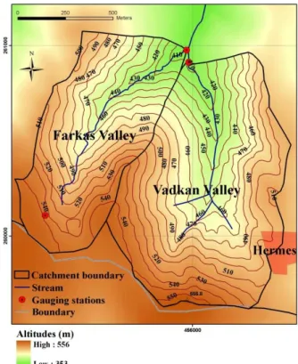
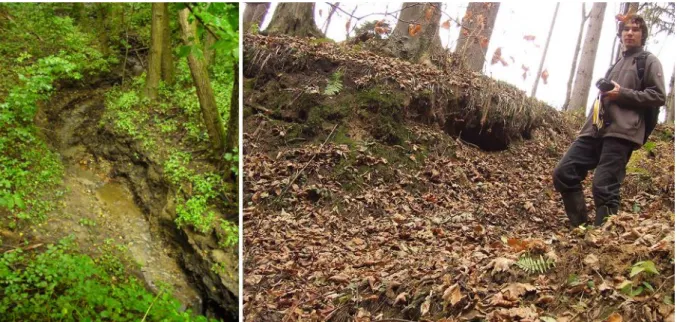
3.1 Study area ... 38
3.1.1 The catchment of the Rák Brook ... 38
3.1.2 The Farkas Valley and the Vadkan Valley ... 39
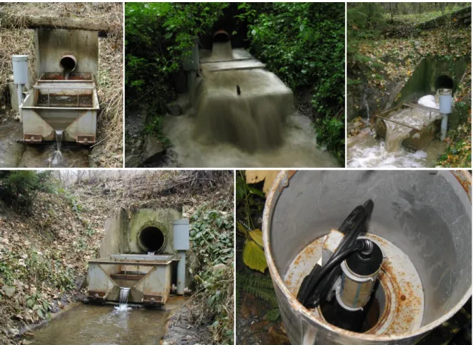
3.2 Sediment and sediment control parameters ... 44
3.2.1 Precipitation data ... 44
3.2.2 Runoff data ... 46
3.2.3 Temperature data ... 48
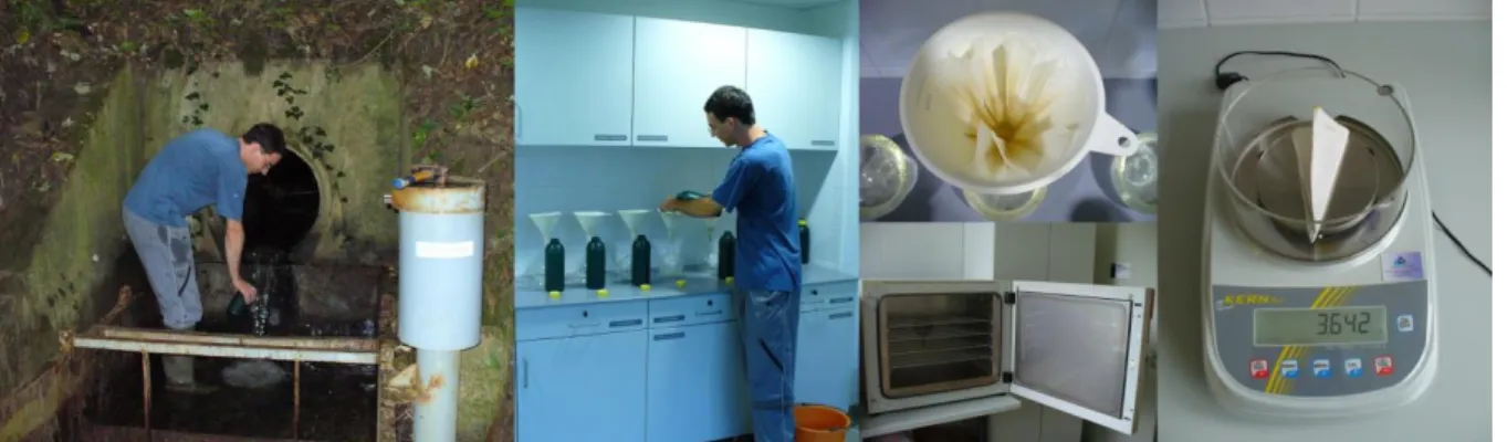
3.2.4 Sediment data ... 48
3.3 Statistical analyses ... 52
3.4 Geodesic survey and working with GIS ... 53
3.5 Soil loss calculations ... 56
3.5.1 Determination of factors of the Universal Soil Loss Equation (USLE) ... 56
3.5.2 Datasets and parameters of the EROSION-3D ... 58
4. Results ... 59
4.1 Soil, rainfall and runoff conditions ... 59
4.1.1 Soil map of the Farkas Valley and spatial distribution of the K factor ... 59
4.1.2 Precipitation categories and the descriptive statistical variables of different rainfall parameters ... 59
4.1.3 Characterization of flood events in the Farkas Valley ... 63
4.2 Suspended sediment concentration and its control factors ... 66
4.3 Relation between suspended sediment and sediment control factors ... 71
4.3.1 Relation between suspended sediment and sediment control factors at low flow ... 71
4.3.2 Relation between suspended sediment and sediment control factors at high flow ... 75
6
4.4 Sediment yield calculations ... 85
4.4.1 Regression equations for calculating suspended sediment yield ... 85
4.4.2 Calculation of sediment yield at annual and event-scale ... 86
4.4.3 Quantification of the sediment contribution by an outwashing sediment deposit ... 91
4.5 Contribution of soil erosion to the sediment transport ... 94
4.5.1 Development of the workflow “Erosion analysis” in the ArcGIS Model Builder ... 94
4.5.2 Modelling of surface erosion with the USLE in the Farkas Valley ... 97
4.5.3 Modelling with EROSION-3D ... 99
5. Discussion and conclusions ... 102
6. Outlook ... 105
7. Theses of the dissertation ... 106
Acknowledgements ... 108
References ... 109
List of figures ... 121
List of tables ... 123
Annex ... 124
Annex I.III ... 124
Annex I.IV ... 125
Annex I.V ... 126
Annex III.I ... 127
Annex III.III ... 131
Annex III.V ... 133
Annex IV.I ... 136
Annex IV.II ... 140
Annex IV.III ... 144
Annex IV.IV ... 148
Annex IV.V ... 152
7
List of symbols and abbreviations
A average annual soil loss (t·ha-1·yr-1)
a, b, c, d, f, j, k, m, n, o, p empirical (rating) coefficients (dimensionless) ABF strongly acidic non-podzolic brown forest soil
Ac catchment area (km2) AC aggregate category
AD antecedent days (number of days elapsed since the previous flood event) (days) API antecedent precipitation index (cumulative rainfall depth) (in general)
API1 antecedent precipitation of 1 day before the sampling/before the flood event (mm) API3 antecedent precipitation of 3 days before the sampling/before the flood event (mm) API7 antecedent precipitation of 7 days before the sampling/before the flood event (mm) BY bedload yield (t·yr-1; t·month-1)
BY* bedload yield between two measurements (kg) BYbf_average average baseflow bedload yield (kg·min-1) BYflood_obs bedload yield of the sampled flood event (kg) C cover-management factor (dimensionless)
CF log-transformation bias correction factor CS colluvial soil
c1 tipping bucket rain gauge with 0.1 mm rainfall capacity D mean stream depth (m)
DEM Digital Elevation Model
ds diameter of sediment particle (mm) e exponential function
EI rainfall erosivity index (kJ·m-2·mm·h-1) g acceleration due to gravity (m·s-2) G specific gravity (dimensionless) GIS Geographical Information Systems h water stage (cm)
hhm tipping bucket rain gauge with 0.5 mm rainfall capacity Imax30 maximum 30-min rainfall intensity (mm·h-1)
K soil erodibility factor (t·ha-1·m2·kJ-1·h·mm-1) L slope length factor (dimensionless)
LBF lessivated brown forest soil LWD large woody debris
MD molecular diffusion coefficient (L2·T-1) m, n empirical exponents
OS content of organic substance (%)
P erosion-control practice factor (dimensionless) PBF podzolic brown forest soil
PC category of permeability q, Q discharge (m3·s-1, l·s-1)
qbv volume of gravel material in motion per unit cross-section width and time (L2T-1) qbv* dimensionless volumetric unit sediment discharge
Qd daily discharge of water (m3·s-1)
Qmax peak discharge during a flood event (l·s-1) Qs sediment yield (mg·s-1)
8 p significance level in the statistical analyses P rainfall depth (mm)
r correlation coefficient (Pearson’s r)
r2 determination coefficient (in linear regressions) R rainfall-runoff erosivity factor (kJ·m-2·mm·h-1) Rh hydraulic radius (m)
s energy slope of the reach (dimensionless) S slope steepness factor (dimensionless) SD, Std.Dev. standard deviation
SDR sediment delivery ratio (%)
SSC suspended sediment concentration (mg·l-1) Ssed suspended sediment supply
ST0 soil temperature at 0 cm depth (oC) ST5 soil temperature at 5 cm depth (oC) ST10 soil temperature at 10 cm depth (oC) SSY suspended sediment yield (t·yr-1)
SSYd daily discharge of suspended sediment (kg·s-1) SumQ total volume of the flood event (l)
SumQhf total volume of high flow periods between two bedload measurements (l) SY sediment yield (in general)
t time/duration
TSY total sediment yield (suspended sediment yield + bedload yield) (t·yr-1) u* shear velocity
USLE Universal Soil Loss Equation x, y, z coordinates
v mean flow velocity in the cross-section (m·s-1) vb actual flow velocity near the bed
vc critical velocity required to just move a particle (m·s-1) W stream width (m)
WT water temperature (oC) Greek symbols:
1,2,3,4, 1,2,3,4 empirical coefficients
slope steepness (o)
specific weight of water (Nm-3)
m specific weight of the fluid mixture (Nm-3)
s specific weight of the sediment particle (Nm-3)
turbulent mixing and dispersive coefficient
mass density of water (kg·m-3)
m mass density of the water-sediment mixture (kg·m-3)
s mass density of sediment (kg·m-3)
standard error of the regression equation
0 shear stress at the bed (N·m-2)
c critical shear stress to initiate gravel motion (N·m-2)
* dimensionless shear stress – Shields parameter
0 Rubey’s clear-water fall velocity
empirical rating parameter (dimensionless)
9
Abstract
The dissertation reveals the complexity of sediment dynamics and describes the reasons of the sediment stochasticity with special regard to the suspended sediment transport in the catchment of the Rák Brook in the Sopron Hills, Hungary. Based on ten-years-long dataset, the relation between suspended sediment concentration and hydrological, hydro- meteorological and meteorological variables has been evaluated at different flow conditions and different temporal resolution in the Farkas Valley and the Vadkan Valley. The results draw attention to the seasonality, the inter- and intra-event fluctuation of the parameters. As sediment outwash and replenishment may explain the low flow sediment dynamics as well, the role of days elapsed since the previous flood event has also been the investigated. As a major result of this part, different hysteresis types have been recognised on the basis of sediment rating curves under high flow conditions.
To calculate suspended sediment concentration under high flow conditions, regression models have been developed. Using the observed and modelled values, sediment yield has been computed at event and annual scale in the Farkas Valley. The reference hydrological year is 2008-2009, in order to point out the influence of a sediment deposit on the total annual sediment yield which has been outwashed between October 2008 and August 2009. The calculated total sediment yield (124.7 t·yr-1) is equal as if about 0.15 mm soil layer eroded from the surface of the entire catchment and reached the channel. As a stochastic process, sediment exhaustion from the deposit behind log jam increased by 15% (15.8 t sediment surplus) the total sediment yield.
Erosion modelling has been performed with an empirical soil loss equation (Universal Soil Loss Equation – USLE, Wischmeier & Smith 1978) and a physical erosion model (EROSION- 3D, von Werner 1995). The USLE modelling, which have been supported by a self-made workflow built in the ArcGIS Model Builder, shows that surface erosion is not an important form of soil erosion in the Farkas Valley (13% proportion to the total annual sediment yield).
The length-slope factor is the most important factor determining the surface erosion. Test of the EROSION-3D model can only be applied for qualitative analyses of soil erosion: the unpaved roads produced the highest average soil loss.
Although several research questions in connection with sediment dynamics in forested catchments have not been clarified yet, the results give new aspects for the sediment transport and erosion processes in the Sopron Hills. Results of the low flow sediment transport and the GIS-workflow to the USLE model can be utilized outside of the study catchment as well. To achieve more plausible and comprehensive results, development of the data collection methods is a necessary requirement in the future.
10
Kivonat
A disszertáció feltárja a hordalékszállítási dinamika komplex jellegét és jellemzi annak sztohaszticitásának okait, különös tekintettel a Soproni-hegységben eredő Rák-patak mellékvízgyűjtőinek lebegtetett hordalékszállítására. A szerző dolgozatában 10 éves adatsor alapján vizsgálja a Farkas-árokban és Vadkan-árokban mért lebegtetett hordalékkoncentrációk összefüggését hidrológiai, hidrometeorológiai és meteorológiai paraméterekkel különböző vízhozam-tartományok és időbeli felbontás esetén. Az eredmények rámutatnak az egyes változók szezonális változására és az egyes árhullámok alatti és közötti fluktuációjára. Mivel a hordalék árhullámok alatti kimosódása és visszatöltődése a kisvízi hordalékszállítás törvényszerűségeit is magyarázhatja, a szerző a megelőző árhullám óta eltelt napok számát is bevonta vizsgálataiba. A dolgozat egy fő eredménye, hogy az árhullámok alatti hordalékkoncentráció és vízhozam közötti kapcsolat (hordalékhozam-görbe) elemzése során több különböző hiszterézistípust sikerült azonosítani.
A szerző regressziós egyenleteket határozott meg a nagyvízi lebegtetett hordalékkoncentrációk számítására. Mért és modellezett értékek felhasználásával kiszámolta a Farkas-árok hordalékhozamát esemény és éves szinten. Referenciaként a 2008-2009-es hidrológiai év szolgált, hogy egy 2008. október és 2009. augusztus között kiürülő hordalékdepónia éves hordalékhozamra gyakorolt hatása is számszerűsíthető legyen. A számolt éves hordalékhozam (124,7 t/év) úgy értelmezhető, mintha a vízgyűjtőről egységesen 0,15 mm talaj pusztult volna le és az mind a patakmederbe került volna. A hordalékdepónia elszállítódása – sztochasztikus folyamatként – 15%-os növekedést okozott a Farkas-árok éves hordalékhozamában (15,8 t hordaléktöbblet).
Az eróziómodellezés egy empirikus talajvesztési egyenlettel (Általános Talajvesztési Egyenlet – USLE, Wischmeier & Smith 1978) és egy fizikai eróziómodellel (EROSION-3D, von Werner 1995) történt. Az Általános Talajvesztési Egyenlet – amelyet a szerző az ArcGIS Model Builder segítségével adaptált térinformatikai környezetbe – alapján a felületi erózió elhanyagolható jelentőségű a Farkas-árok területén (13%-os részesedés az éves hordalékhozamból). Az eróziót leginkább meghatározó tényező a lejtés-lejtőhossz faktor. Az EROSION-3D modell csak a talajpusztulás minőségi értékelésére volt alkalmazható. E modell szerint a burkolatlan közelítőutak produkálták a legmagasabb átlagos talajveszteséget.
Habár a disszertáció számos tudományos kérdésre nem ad választ, eredményei mégis egy új irányvonalat jelentenek a Soproni-hegység hordalékszállításának és talajpusztulásának vizsgálatában. A kisvízi hordalékszállítással kapcsolatos következtetések és az USLE modellhez elkészített GIS-keretrendszer pedig más vízgyűjtőkön is alkalmazhatók.
Megbízhatóbb eredmények és átfogóbb megállapítások elsősorban az adatgyűjtési módszerek jövőbeli fejlesztésével lennének elérhetők.
11
1. Introduction
1.1. Background
Nowadays sediment transport and soil erosion processes may lead to even more serious environmental and ecological catastrophes due to the global climate changes. Precipitation scenarios for Hungary agree that intensity and frequency of extreme precipitation will increase, while the total precipitation amount will decrease. Namely the change of rainfall distribution leads to the increase of drought and heavy rainstorm frequency (Bartholy &
Pongrácz 2007, Gálos et al. 2007, Kis 2011). The intensification of rainfall events accompanies the increase of surface runoff due to the time reduction of infiltration and infiltration excess. As the hydrological response will be faster, the rise of design flood level is also expected, especially in the small catchments. Higher raindrop energy, surface runoff and stream power have influence on the rate of soil detachment and transported SY as well.
Several news and studies reported on disastrous flash floods and debris flows when not only the high Q but the meaningful SY was also responsible for the damages (URL1-3, Vinet 2008, Mizuyama & Egashira 2010, Shieh et al. 2010).
Soil erosion, as the main source of the sediment in the watercourses shows also a growing tendency related to the extreme precipitation. However, the role of the land use is also important considering the sediment delivery problem. Although water erosion is a natural process which is responsible for landscape degradation (Thyll 1992), human activities, such as road building, tree and crop harvesting and overgrazing increase the detachment of soil particles. Soil loss promotes different harmful hydrological changes in the soil (e.g. reduction of water holding capacity, infiltration capacity) and in the water bodies as well (e.g. decrease of river channel stability and siltation of channels and lakes). The decreasing reservoir capacity and flow section of channels imply higher flood risk (Lewis 1998). Changes of channel morphology may cause the loss or modification of aquatic habitats. Eroded material as suspended sediment enhances the turbidity altering the aquatic ecosystems (Ma 2001).
Suspended particles can directly injure gills of fish and macroinvertebrates, impair the ability to locate food, reduce the depth at which photosynthesis can take place. Suspended particle- bond substances can lead to the contamination of aquatic ecosystems, such as eutrophication caused by the nutrients (Clement et al. 2009, Rodríguez-Blanco et al. 2009a) and acute intoxication due to contaminants, such as metals (Rodríguez-Blanco et al. 2009b). Sediment in the water shortens the life of irrigation systems and hydraulic structures. To avoid the multiple harmful effects, as reported by several authors (Bogárdi 1971, Shen & Julien 1993, Gordon et al. 2004, Owens & Collins 2006, Chang 2006), it is necessary to get detailed information about soil erosion and sediment dynamics. Nevertheless, it is a difficult question to predict sediment motion and to plausibly calculate SY for the future, because the sediment dynamics shows significant spatial and temporal fluctuation.
12
The preceding researches related to the soil erosion in forested catchments were performed by the Hungarian Forest Research Institute in the Mátra Mountains (Bánky 1959, Újvári 1981).
They measured soil loss at plot-scale in different forest stands.
To calculate average soil loss and life expectancy of forest ponds, and to describe the complex dynamics of bedload and suspended sediment transport sediment researches also started in the forested catchments of Sopron Hills (Kucsara & Rácz 1988, Kucsara & Rácz 1991, Gribovszki & Kalicz 2003). To determine bedload yield (BY) and suspended sediment yield (SSY), Gribovszki (2000b) developed regression equations.
1.2 Soil erosion by water
The importance of soil erosion is well represented thereby creating the erosion maps and water management maps of Hungary (Duck 1955, Stefanovits 1964, Kazó 1970, Kerényi 1991), and including the regular soil loss measurements into the Hungarian National Information and Monitoring System for Soil Protection as a subsystem of the integrated Information and Monitoring System for Environment Management (Várallyai 1992, Nováky 2001).
Knowledge about the different erosion forms is important, in order to select the adequate model for soil loss prediction. A classic categorization basis of soil erosion types is the agricultural practice and the cultivability of plot after erosion. I describe the different types of soil erosion by water according to Stefanovits et al. (1999, ps. 328-331.) and URL4 below.
Inter-rill or surface erosion: Soil loss phenomena within a plot which do not limit the horizontal (following the contour-lines) cultivation. Soil detachment occurs in a layer with homogeneous depth which remains under the tillage depth. Scales of the surface erosion are:
Micro-solifluction: This form is generally invisible. It appears when more rainfall reaches the saturated soil surface which goes into a suspension with the runoff and begins to slide slowly downstream to a point of deposition in a very thin layer but at large extension.
Splash erosion: This phenomenon is induced by the hitting impact of raindrops. The effect is different on dry and wet soil surface (explosive and splashing effect).
Sheet erosion: This form appears due to the unconcentrated surface runoff when soil particles start to move at large extension at the same time.
Rill erosion: This type occurs when sheet flows and smaller flow paths on the soil surface start to converge into larger water rills. Its effect is not uniform leaving visible scouring on the surface. Damages cannot be corrected by shallow tillage, but the horizontal mechanical cultivation has been possible yet. The reasons can be: e.g. wheel-tracks, furrows etc.
Gully erosion: Rill erosion evolves into gully erosion as duration or intensity of rain continues to increase and runoff volumes continue to accelerate. A gully is generally defined as a scoured out area that is not crossable with tillage or grading equipment. Thus, farming activities are impeded by gully erosion (Duck 1969, Stefanovits 1999).
13
Although afforestation can stabilize gully development (Gábris et al. 2003), studies of Jakab et al. (2005) and Jakab (2008) draw the attention that gully erosion can occur in catchments with mixed land use or forested regions as well. Similarly in the Sopron Hills, primarily the rills and gullies are dominant (due to the unpaved forest roads), as for the runoff-driven erosion. However, quasi-invisible surface erosion forms can also appear in some regions where the forest cover had been removed. Besides the soil loss by water runoff, gravity combined with other forces such as soil saturation, earthquake and uprooting can lead to different mass movements on steep hillslopes.
Without giving detailed descriptions of mass movements and their driving forces, some examples are listed here. In the model of Benda & Dunne (1997), complex interaction between climatic and topographic factors had been embedded which influence the slope stability and may trigger landslides. These elements are: fire regime – root strength, precipitation regime – pore pressure in colluvium, depth of colluvium, soil strength and topography. Water can induce the downslope movements of surface material in several ways (URL5):
adding weight to the soil,
filling the pore spaces of slope material,
exerting pressure which tends to push apart individual grains.
Landslide is a general term which can be divided into the more specialized categories, such as slump, rockslide, debris slide, mudflow and earthflow.
Sediment delivery ratio. Researches introduce that only a small fraction of the soil eroded within a basin will reach the catchment’s outlet, and sediment sources of a stream are not necessarily the major soil erosion areas because different parts of a catchment has different transport capacity to convey sediment. Particles can be deposited and temporarily or permanently stored on the slope, particularly where gradients reduce downslope, at the base of the slope, in swales, on the floodplain or in the stream channel (Walling 1983, Di Stefano et al. 2000). In order to assess sediment yield (SY) from soil loss it is necessary to estimate the SDR and the time lag between basin SY and soil erosion as well (Ferro & Minacapilli 1995, Amore et al. 2004). The residence time of sediment in the storage elements towards the base level may increase from decades to 10000 years (Dietrich & Dunne 1978).
Nevertheless, SDR varies within a catchment, depending on geomorphological and environmental factors such as extent and location of sediment sources, relief, drainage network and channel conditions, land cover, land use and soil types (Walling 1983). Many authors investigated the sediment delivery problem applying empirical, statistical, physical respectively spatially lumped and distributed SDR equations (Ferro & Minacapilli 1995, Di Stefano et al. 2000). But in the frame of this study, only the empirical equation of Vanoni (1975, in Lim et al. 2005) is highlighted. The principle of this formula is the relation between catchment area (Ac, km2) and SDR (“SDR curve”):
125 0 4724
0. A .
SDR c (Eq. 1.1)
14 1.3 Soil erosion modelling
Many models have been developed to predict areas sensitive to water erosion, to predict soil loss, and to evaluate soil erosion-control practices. They can be classified in different ways, e.g. according to
calculation method (empirical, semi-empirical, physical),
spatial resolution (lumped or distributed) and extent of spatial units (plot-scale, slope- scale, watershed-scale),
temporal resolution (event-based, continuous – integrated estimation for a given time period),
pollution sources (non-point or point-source pollution, soil loss, nutrients),
processes (erosion, deposition, sediment transport).
Annex I.III.1 shows examples of the different types of erosion models. Since the author applied the empirical equation of Universal Soil Loss Equation (USLE, Wischmeier & Smith 1978) implemented in GIS-environment and the physical-based model of EROSION-3D (von Werner 1995), following descriptions involve these models.
1.3.1 The Universal Soil Loss Equation and its applicability
In contrast with physically based models, Martin et al. (2003) noted that empirical models such as the USLE require less site specific data. Therefore, the USLE is more widely applied for predicting soil loss and for planning of soil conservation measurements, especially in developing countries (Szabó 1995, Jain & Kothyari 2000, Lu et al. 2004, Onyando et al.
2005, Erdogan et al. 2007, Pandey et al. 2007). The USLE is an empirical equation originally developed by Wischmeier & Smith (1978) in the USA. The Hungarian adaptation had been performed by Kiss et al. (1972, in Salamin 1982), while Schwertmann et al. (1987) elaborated the application in Germany. The equation computes the average specific soil loss pro unit area by multiplying the following six factors:
P C S L K R
A , where (Eq. 1.2)
A is the average annual soil loss (t·ha-1·yr-1);
R is the rainfall-runoff erosivity factor (kJ·m-2·mm·h-1) which represents the erosion potential of locally expected rainfalls on cultivated soil without vegetation cover;
K is the soil erodibility factor (t·ha-1·m2·kJ-1·h·mm-1) which shows the rate of soil loss per unit of rainfall for a specific soil for a clean-tilled fallow;
L is the slope length factor (dimensionless), the rate of soil loss compared to the soil loss from a 22.13 m length slope;
S represents the slope steepness factor (dimensionless), the rate of soil loss compared to the soil loss of a slope with a 9% inclination;
C is the cover-management factor (dimensionless) which shows the influence of plants in contrast with bare fallow;
P is the erosion-control practice factor (dimensionless) where control practices are usually contours, strip cropping or terraces (Centeri 2001, Amore et al. 2004).
15
Dettling (1981) and Centeri (2001) drew the attention to the importance of the proper harmonization of American and SI units at the European USLE adaptations. The calculated soil loss can be compared to the tolerable soil loss which indicates the maximum level of soil erosion that still allows a high level of crop productivity over the years (Stone & Hilborn 2000).
Many authors discussed the applicability of the USLE in different study areas. Originally, the USLE allows the long term prediction of soil loss only for standardised agricultural plots (Wischmeier & Smith 1978, Schwertmann et al. 1987). The adaptation of the equation to a wider scale and to other land usages (e.g. forest) is not recommended by Wischmeier & Smith (1978). The predicted soil loss may exceed the observed values by one order of magnitude in forested areas (Risse et al. 1993). The reasons of the overestimation can be that the soil distribution is mostly irregular and surface runoff is often prevented by organic debris such as logs, twigs and leaves. In addition, the rate of macropore infiltration is also high (Gribovszki ex verb.). However, several other authors proved that USLE is capable for estimating soil loss under different conditions (Jain & Kothyari 2000, Onyando et al. 2005, Khosrowpanah et al.
2007, Beskow et al. 2009). Rácz (1985) suggested factor values to the USLE adaptation in forested catchments of Hungary.
Considering the C factor, the international studies give a wide range of its value even for the similar land cover types. Wischmeier & Smith (1978) classifies the C factor according to the canopy type and height, the % cover by the vegetative canopy and the cover that contacts the soil surface. Minimal C factor is 0.003 independently on the canopy, if the cover consists of grass, grasslike plants or decaying compacted litter, and ground cover is higher than 95%.
However, C factor is not lower than 0.011, if the cover consists of broadleaf herbaceous plants and undecayed residues. In case of 75-100% canopy or undergrowth cover and 90- 100% litter cover, C factor can decrease to 0.0001 in forested catchments. Some authors agree that mean annual C factor has 0.1 orders of magnitude for different crop rotation systems (Márkus & Wojtaszek 1993a, Gabriels et al. 2003, Tetra Tech 2007, Khanal & Parajuli 2013). Schwertmann et al. (1987) specify “advantageous” cases when C factor can be 0.01 orders of magnitude on arable land as well. Furthermore, mulch cover can also reduce the values. This value is 0.001 order or magnitude in forests or pasture (Khanal & Parajuli 2013).
Other authors work with higher values for the pasture: 0.01 order of magnitude in Ma (2001) and Tetra Tech (2007). In the study of Kosky (1999), cropland, forest and wetland have C factor in the same order of magnitude contradicting the previous researches relating the croplands. Some researchers distinguish C factor in deciduous and evergreen/coniferous forest, where evergreen/coniferous forest produces almost by 50% lower values than deciduous forests (Ma 2001).
The USLE had been developed for the prediction of sheet and rill erosion. However, the results show no separate values for rill and inter-rill erosion, but overall soil loss only. The USLE is also not feasible for estimating the amount of deposition and for calculation of sediment yield (SY) from gully, streambed and streambank erosion (Wischmeier & Smith 1978, Fistikoglu & Harmancioglu 2002). The equation was primarily designed for calculating
16
long-term average annual rates of erosion (Stone & Hilborn 2000). It is therefore necessary to develop techniques to estimate soil loss for individual storm events (Jain & Kothyari 2000).
Andersson (2010) noted that interactions between USLE factors are not taken into account.
1.3.2 Implementation of the USLE in Geographical Information Systems
Soil erosion risk differs spatially because of heterogeneous topography, geology, geomorphology, soil types, land cover, and land use. Geographical Information Systems (GIS) are able to handle these spatially variable data easily and efficiently. The estimation of soil erosion with GIS techniques reduces costs and improves accuracy (Ma 2001, Erdogan et al. 2007, Khosrowpanah et al. 2007). State-of-the-art GIS provides the necessary mapping and interpolation methods to create a database, which includes all input datasets for erosion modelling. The resolution should reflect the spatial variation of the hydrological and erosion processes (Fistikoglu & Harmancioglu 2002, Beskow et al. 2009). Decreasing cell size and increasing scale requires a large amount of data for accurate prediction. GIS is therefore most appropriate for the management of a huge amount of data. It reduces time and costs for accessing and handling a database (De Roo & Jetten 1999). De Roo et al. (1996), Fistikoglu &
Harmancioglu (2002), Khosrowpanah et al. (2007), and Pandey et al. (2007) described even more advantages of GIS, such as the production of complex input maps and the combination of soil, land use and coverage information. With GIS techniques, the calculation of soil loss rates for alternative land management scenarios becomes easier.
The required data for the prediction of soil loss (rainfall erosivity, soil data, digital elevation model, land use) has to be converted into a GIS-format in order to implement the USLE in GIS. Different authors have used GIS-based techniques to model USLE factors for predicting soil loss for larger watersheds on a grid cell basis (Erdogan et al. 2007, Andersson 2010).
According to Martin et al. (2003), a combined USLE/GIS approach is able to identify discrete locations with precise spatial boundaries with high erosion potential. Beskow et al. (2009) validate that the combined USLE/GIS technique shows an acceptable accuracy and allows mapping of the most susceptible areas. The studies by Onyando et al. (2005) and Erdogan et al. (2007) contradicted this: upscaling of the USLE-applications from plots to large watersheds is limited depending on the reliability and availability of direct field measurements. As Fistikoglu & Harmancioglu (2002) mentioned, the results of erosion risk assessment are more plausible for small grid sizes and smaller areas. Therefore larger watersheds must be analysed as sub-basins. A comprehensive USLE/GIS application was accomplished in the frame of the Balaton Project in Hungary, where Kertész et al. (1992, 1997) divided the Örvényes Catchment into “erotopes” which indicate the inclined parts of the relief with an unconcentrated runoff approximately in the same direction. This technique ensures to analyse the impact of unconcentrated runoff and to model soil erosion in a larger catchment at quasi-plot scale or in slope segments.
The combined USLE/GIS approach is also limited by each input factor. Auerswald (1987) stated that the calculated soil loss is highly sensitive to the slope factor. To provide a more
17
accurate slope length prediction, the ArcInfo Arc Macro Language (AML) scripts of Van Remortel et al. (2001) calculates the cumulative uphill length from each cell. All convergent flow paths and depositional areas are integrated in this model. Van Remortel et al. (2004) presented another GIS-model based on the revised USLE. The AML processing code solves the difficulty in obtaining the LS factor grid at regional scales using ANSI C++ software.
Modern GIS-based procedures support the calculation of other USLE factors as well. Many studies applied remote sensing data to develop values for the C and P factors, to classify land cover categories and land use units (Ma et al. 2003, Beskow et al. 2009). These studies confirmed that the original spatial limitations of the USLE can be avoided by using remote sensing data and GIS. Márkus & Wojtaszek (1993a, 1993b) conducted the USLE calculation in ArcInfo environment and compared the density differences of aerial photographs and satellite images with the erosion sensitive areas. The results proved that remote sensing is a suitable method to check the modelled soil erosion categories and to follow the actual stage of the erosion processes.
According to the literature overview, integration of GIS-based techniques with the USLE is useful to describe areas that are vulnerable to soil erosion, enabling immediate conservation planning (Lee 2004, Beskow et al. 2009).
1.3.3 The soil erosion prediction model EROSION-3D
EROSION-3D (von Werner 1995) is a process-based model, which means that it predominantly operates based on physical principles of the following erosion processes:
runoff generation;
particles detachment by raindrop impact and runoff;
transport of eroded particles by runoff;
routing of runoff and sediment through the catchment;
sediment deposition.
The model considers critical shear strength of the soil and transport capacity of the runoff as physical principles of the particles detachment and transport, which are expressed in a form of a critical momentum flux. Rainfall infiltration excess is calculated by the modified Green &
Ampt equation, which shortcoming is the reliable simulation of macropore flow.
The model works on the basis of a regular grid where the grid size is variable, but must be consistent within a matrix of a catchment (more than 5·105 raster cells). The model operates on an event basis, and the temporal resolution ranges from 1 to 15 min. Grid-based processing requires the model applicability in Geographical Information Systems (GIS) (e.g. ArcInfo, GRASS) (Schmidt et al. 1999).
Figure 1.1 represents the model structure referring also to the calculation process. Input parameters are described in Sect. 3.5.2. The model consists of two modules, the GIS and the erosion component. The GIS module performs the preprocessing of Digital Elevation Model (DEM), generating the flow direction and flow accumulation for each grid and creating the
18
channel network. The erosion component determines the rate of surface runoff and soil loss.
In detail, EROSION-3D is able to calculate:
erosion and deposition by rill and inter-rill erosion;
particle transport and deposition for nine soil fractions from fine clay to coarse sand;
sediment volume and sediment concentration in the channels’ grid.
Figure 1.1. Model structure of the EROSION-3D (from Kitka 2009)
Thus, EROSION-3D enables to analyse the effect of erosion-control practices (e.g. changes in the agricultural techniques and plants), the sediment retention in basins and ditches, nutrient inlet to the streams through soil particles, snowmelt erosion, etc. (Kitka 2009).
Nevertheless, EROSION-3D has also several shortcomings. Besides the high data requirements and quantitative overestimation due to the neglected macropore flow and surface crusting, reliability of qualitative and quantitative soil loss prediction from linear erosion (rill erosion) is limited as well. For instance, as Bug (2011) found, modelling the location of erosion forms was not entirely accurate. The model indicated soil loss reduction in a thalweg, but the field observation proved high erosion damages in that place.
19 1.4 Sediment types
Physical and chemical weathering plays a major role in the decomposition of bedrock. The products of weathering, such as smaller particles, soil minerals and dissolved constituents, are removed by erosion processes, where the main agent is the water. Since residual materials formed by weathering are usually eroded and transported to the streams, water quality is also influenced by erosion processes (Bricker et al. 1992). Sediment in streams can be classified in many different ways. In order to describe sediment in general, total sediment yield can be categorized as bedload and suspended sediment. Bedload has an almost permanent contact with the streambed while moving, and suspended sediment is in suspension (Bogárdi 1971).
The threshold distinguishing bedload from suspended load depends on the particle size and flow magnitude. In the technical practice only fractions larger than 0.002 mm are reckoned as sediment. One of the sediment classification methods separates sediment types according to the origin. Sediment in the streams comes from the slopes of watershed (washload) or the channel itself (bed-material load), where washload contains particles are finer than the bed- material.
Considering the several different types of sediment movements, origins and other characters the following complex classification has been defined. Total sediment yield of the stream is the amount of dissolved and particulate organic and inorganic material. Although there are no sharp boundaries, total load can be divided into three groupings: flotation load, dissolved load, sediment yield (Figure 1.2) (Gordon et al. 2004).
Figure 1.2. Classification of the transported material in streams (from Gordon et al. 2004)
Logs, leaves, branches and other organic debris, which are generally lighter than water, compose the flotation load. The organic debris is supplied from the vegetation along the banks, bank failure and tree fall. The dissolved load is the material transported in solution.
Origins of dissolved load can be the sea salts dissolved in the rainwater, the chemical weathering of rocks – sometimes enhanced by organic acids from the decay of vegetation, industrial effluents and agricultural solutes. Sediment, which is usually considered to be the solid inorganic material load according to Gordon et al. (2004), can be further separated into the following categories: washload, bed-material load, which can be transported as suspended load or bedload.
Washload refers to the smaller sediments, primarily clays, silts and fine sand fractions washed into the stream from the banks and upland areas. The size ranges from 0.0005 mm to 0.0625mm, where the smallest grain size is the distinguishing value between dissolved load
20
and washload. Only low velocities and minor turbulences enable that washload may never settle out, and its concentration is considered constant over the depth of a stream. As Hjulstrom (1939, in Gordon et al. 2004) said, streams cannot become saturated with sediment as they can with dissolved solids. High washload concentration may typify streams with banks of high clay-silt content, and catchments after fire denudation, volcanic eruptions, road or dam building and agricultural practices.
Bed-material load is the material in motion which has approximately the same size range as the streambed particles. Depending on flow conditions, the portion of bed-material load remaining in suspension for an appreciable length of time is called suspended bed-material load. Bedload is that portion which moves by rolling, sliding or ‘hopping’ in a narrow region near the bottom of the stream. Based on the method of data collection, washload and suspended bed-material are often grouped into the single category, suspended load. Another conventional separation of suspended load from bedload is based on the sand particle size threshold at 0.0625 mm. However, this threshold value may differ according to other authors.
According to the review of Gomi et al. (2005) sediment particles carried in suspension are fine sand, silt and clay with the diameter less than 0.2 mm. Nevertheless, depending on flow magnitude, particles which have diameters 0.2 to 2 mm may move either in suspension or as bedload. Particles which are finer than sands tend to be evenly distributed in the cross-section, while coarser material is more concentrated near the bed (Julien 2010).
This dissertation follows the general sediment separation and discusses bedload and suspended sediment forms. Although bedload can play a major role in the alteration of channel geometry and destruction of water structures, this work focuses primarily on the suspended sediment transport, because generally less bedload than suspended load is transported over a year. The ratio of bedload to suspended load is in the range 1:30 to 1:40 in summer and 1:2 to 1:3 in winter in the headwater catchments of the Rák Brook (Gribovszki 2000a).
1.4.1 Bedload transport
Principles of incipient sediment motion. Stream power describes the erosive capacity of streams, and it is related to the shape of the longitudinal profile, channel pattern, the development of bed forms and sediment transport. According to the Bagnold’s definition (1966, in Gordon et al. 2004), stream power
per unit of streambed area is equal to (N·m-1·s): a 0v (Eq. 1.3) per unit of stream length (kg·m·s-3): l gqs (Eq. 1.4) per unit mass of water (m2·s-3): m gvs (Eq. 1.5) per unit weight (m·s-1): a 0v (Eq. 1.6) In the equations, 0 is the shear stress at the bed (N·m-2); v is the mean flow velocity (m·s-1) in the cross-section; is the density of water (kg·m-3); g (m·s-2) is the acceleration due to gravity;
q is the discharge of water (m3·s-1); s is the energy slope of the reach (dimensionless). l is also called total stream power in the literature.
21
Leopold & Maddock (1953, in Gordon et al. 2004) found that hydraulic geometry of a channel varies with the streamflow, and the changes can be well demonstrated by the following relationships:
Qb
a
W DcQf vkQm Qs pQj, (Eq. 1.7)
where the unknown units are: Q is the discharge (l·s-1); W is the stream width (m); D is the mean depth (m); Qs is the sediment yield in a given time-period (mg·s-1); a, b, c, f, k, m, p and j are empirical coefficients.
Lift and drag forces act on a sediment particle when pressure and velocity differences exist from top to bottom or front to back of the grain. The Hjulstrom curves describe the critical velocities required for particles detachment, transport and deposition; however, they are only valid for idealized conditions (uniform material, D>1m). Jowett’s relative bed stability defines the suitability of a streambed, as the ratio of the critical velocity required to just move a particle (vc) to the actual flow velocity near the bed (vb).
Bedload equations. Bedload indicates the transport of sediment particles which frequently maintain contact with the bed, where the bed layer thickness is the double of the grain diameters as commonly used. Bedload delivery can be treated as a deterministic and probabilistic problem as well. Deterministic approaches are the equation of Du Boys and Meyer-Peter Müller, while the probabilistic equations were developed by Kalinske and Einstein. In the followings, basic bedload equations are overviewed according to Bogárdi (1971) and Julien (2010). Since the dissertation discusses mainly the suspended sediment transport, further bedload equations can be found in the Annex I.IV.1.
As the beginning of theoretical development of the bedload movement can be considered the Du Boys equation (1879, in Julien 2010) which is based on the concept that sediment moves in thin layers along the bed. The applied bed shear stress 0 must exceed the critical shear stress c to initiate motion, where
s Rh
0 , and (Eq. 1.8)
c c ds s , where (Eq. 1.9)
is the specific weight of water (Nm-3); 1 is the specific weight of the sediment particle (Nm-3); Rh is the hydraulic radius (m); c is a constant; ds is the particle size (mm).
The volume of gravel material in motion per unit cross-section width and time equals (qbv; L2T-1):
s
/ s
bv . . d
d
q 0.173 001250019
0 4 0
3 . (Eq. 1.10)
According to the Du Boys theory, only the bed shear stress is accounted for the gravel mobilisation. However, internal power of the stream can also contribute to the bedload transport (Bogárdi 1971).
Shields (1936, in Bogárdi, 1971) substituted the c constant in Eq. 1.9 with a nonconstant resistance coefficient which depends on the Reynolds number. Therefore, the resistance coefficient and the critical shear stress depend on the viscosity and the water temperature as
22
well. It means that the critical shear stress related to a sediment particle, with ds gravel diameter and s density, will increase if the water temperature decreases.
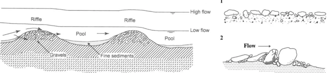
Processes and phenomena influencing the bedload motion. Particle-size distribution and channel features may influence the grain movement. The pool-riffle sequences are most common bedforms in streams with mixed bed materials, where the pool is a region of deeper, slower-moving water, whereas the riffle is a region with shallower, faster-moving water (Figure 1.3). Due to the differences of shear stress in pools and riffles, fine bed materials are concentrating in pools, while coarser particles mostly appear in riffles. Sediment from riffles is mobilized only under large floods, at which time the coarse bed materials are transported from riffle to riffle. However, very coarse fragments will still remain or accumulate in the deepest region of pools (Gordon et al. 2004).
Armouring and imbrication are also accounted for the intermittent character of bedload movement (Figure 1.3). Armouring is the development of a surface layer that is coarser than the bed material beneath it. If the streambed is armoured, the sub-surface particles are protected from channel erosion until the armour layer is broken up. Particle imbrication, which also induces that higher shear stress is required to mobilize the gravels, can occur in streams primarily with disc-shaped pebbles, where particles are stacked against each other, nose-down into the oncoming current. This kind of accumulation may happen because of a sudden fall in the stream’s transport capacity when particles tend to be deposited in their position of transport (Gordon et al. 2004).
Figure 1.3. Channel bed features contributing to the postponement of bedload yield: pool-riffle sequences (left), armouring (1) and imbrication (2) (right) (from Gordon et al. 2004)
If the shear stress or flow velocity exceeds the critical values, e.g. during large flood events, delaying bedload yield (BY) can show a sudden increase due to the following reasons (Gribovszki 2000b):
breaking up of the armour layer on a long stream section,
exhaustion of sediment deposit behind obstructions after their disruption,
changes of the channel geometry,
connection of floodplain sediment sources to the stream channel.
23 1.5 Suspended sediment transport
1.5.1 Physical principles of the suspended sediment transport
The condition of finer particles delivery in suspension is that turbulent velocity fluctuations have to be sufficiently large to maintain the particles within the mass of fluid without frequent bed contact. This subsection sums up the physical principles according to Julien (2010) and Bogárdi (1971). The general physical processes governing the conservation of suspended sediment mass are advection, molecular diffusion, mixing and dispersion. From the sediment continuity equation:
terms _ mixing _ and _ diffusive
z y
x change
_ phase terms
_ advective
y z x
change _ mass
z SSC z
y SSC y
x SSC MD x
z SSC SSC v y
SSC v x SSC v t
SSC
(Eq. 1.11)
In Eq. 1.11 SSC is the suspended sediment concentration (mg·l-1); t is the time; MD is the molecular diffusion coefficient (L2·T-1); is the turbulent mixing and dispersive coefficient; x, y and z are coordinates. “Phase change” includes possible internal mass changes such as chemical reactions, phase changes, adsorption, dissolution, flocculation, radioactive decay, etc.
The advective fluxes describe the sediment transport by velocity currents. Molecular diffusion indicates the scattering of sediment particles by random molecular motion according to the Fick’s law. Turbulent mixing generates the particles motion due to turbulent fluid motion, which effect is by three orders of magnitude higher than the molecular diffusion. Therefore, the molecular diffusion can be neglected.
Regarding the viscosity/temperature-dependency of suspended sediment motion, other relation can be determined. At bedload transport, increasing viscosity induces the stream energy decline due to the thickening laminar layer near the streambed, thus gravel motion will decrease. In contrast, finer particles concentration will decrease according to the temperature dependency of Stokes law, if the temperature declines (Bogárdi 1971).
1.5.2 Temporal variability of the suspended sediment transport
Sediment availability in the channel plays a major role in the suspended sediment dynamics.
Sediment availability is determined by the hydrological parameters, such as the catchment characters and the climatic variables (Bogárdi 1971). Due to the spatial and temporal variability of the hydrological parameters, suspended sediment yield (SSY) shows fluctuation as well. As Walling (1983) summarized, problems of temporal lumping or aggregation can be viewed ranging from the single storm through to a long-term perspective of the erosion–
delivery–sediment yield system. Furthermore, problems of the spatial resolution relate to the accurate representation of the sediment transport characteristics within a basin: the spatial diversity of topographic, land use and soil conditions. This session gives an overview how the
24
suspended sediment transport varies at different time scales and at different flow conditions, and which factors can be accounted for the changes.
Temporal variations occur over a wide range of time scales, and the SSY can vary over a number of orders of magnitude at any one discharge (Q) in the same stream according to Morehead et al. (2003). Albert (2004) and Gao et al. (2011) investigated the long-term sediment time series of large rivers (Rio Grande and Yellow River) using breakpoint analyses, and pointed out that human activities, such as terrace building, dam and reservoir construction, afforestation and grass planting were the main factor for the transition of suspended sediment transport during the studied decades.
Morehead et al. (2003) listed more reasons, which can lead to the intra-annual variability of suspended sediment flux. These are the seasonal changes of water sources (rain versus snowmelt), the altering channel morphology due to the changing climatic conditions, variability of the sediment supply processes and the unstable availability of the fine material in the channel. The authors emphasized that suspended load on smaller rivers tend to have smaller annual variations, and the alteration is smaller on snowmelt-dominated rivers than on rain-dominated basins. The latter statement is also confirmed by Lenzi & Marchi (2000).
Nevertheless, they pointed out that SSY has also noticeable differences depending on the timing and extent of snow cover and snowmelt. Early snowfalls combined with permanent snow cover throughout the winter and slow snowmelt without important rainfall led to negligible SSY, while snowmelt periods which followed a mild winter and late snowfalls caused abundant SSY. According to Alexandrov et al. (2007), the different rainfall types can also be accounted for the inter-seasonal variability of the SSY. Convective or convectively- enhanced storms with high intensity generally led to higher SSC, while the frontal rainfalls with long duration but low intensity induced comparatively lower SSC.
Bronsdon & Naden (2000) have analysed the monthly fluctuation of suspended solid concentration on three rivers in Scotland and identified the control factors. The processes, influencing the amount of easily available fine material in the channel month by month, can be wetting and drying of the catchment, cattle trampling, diatom growth and death, sediment exhaustion, erosion protection by the snow cover, freeze-thaw action, ice-crystal growth along the river banks.
Duvert et al. (2010) found, the analysis of sub-daily (or inter-event) variability of sediment fluxes in small mountainous catchments is inevitably necessary for the accurate calculation of annual SSY. They reported that between 63 and 97% of the annual load is exported in 2% of time, and strong bias (i.e. up to 1000% error) were obtained on annual SSY estimation based on daily sampling due to the very short hydrologic response (1-3 h) of the small catchments (3-12 km2). The significance of event-based suspended sediment sampling in small streams is also confirmed by other authors. Thomas (1985) wrote in his methodological study that most suspended solids are transported during infrequent high flows that are generally underrepresented by the manual sampling strategies. It is not a specific case when the 15% of total Q transfers the 50% of the total SSY in 2% of the reference period. Estrany et al. (2009)