DESIGN OF MEASURES FOR SOIL EROSION CONTROL AND ASSESSMENT OF THEIR EFFECT ON THE REDUCTION OF PEAK FLOWS

DOI: 10.1556/606.2018.13.3.20 Vol. 13, No. 3, pp. 209–219 (2018) www.akademiai.com

DESIGN OF MEASURES FOR SOIL EROSION CONTROL AND ASSESSMENT OF THEIR EFFECT

ON THE REDUCTION OF PEAK FLOWS

1 Marija Mihaela LABAT, ² Lenka KORBEĽOVÁ, ³ Silvia KOHNOVÁ

4 Kamila HLAVČOVÁ

1,2,3,4

Department of Land and Water Resources Management Faculty of Civil Engineering, Slovak University of Technology in Bratislava

Radlinského 11 810 06 Bratislava, Slovakia

e-mail: ¹marija.labat@stuba.sk, ²lenka.korbelova@stuba.sk, ³silvija.kohnova@stuba.sk

4kamila.hlavcova@stuba.sk

Received 24 December 2017; accepted 15 May 2018

Abstract: The aim of this paper is an assessment of the susceptibility of soil to soil erosion, proposed measures against soil erosion, and an assessment of their effect on the reduction of peak flows. The area of interest is the Halúzníkov Creek basin. The calculations of the soil loss from water erosion were done using the universal soil loss equation and universal soil loss equation 2D methods; for estimating design floods, the curve number method was applied. For reducing the soil loss to tolerance values, strip cropping measures on agricultural fields were proposed. After applying the strip cropping measures, the design flood peaks were also reduced.

Keywords: Soil erosion by water, Soil loss, Universal soil loss equation, Universal soil loss equation 2D, Curve number method

1. Introduction

Soil erosion is a complex natural process that cannot be completely prevented, but only reduced to an acceptable or tolerable level. It is one of the most widespread forms of soil degradation [1], which directly affects agricultural land by redistributing soil particles, transporting particles from fields, destroying the soil structure, and reducing the organic matter in the soil. These effects lead to a smaller amount of productivity from agricultural land. Recent policy developments formulated by the European Commission have called for quantitative assessments of soil loss intensity at the European level [2]. Furthermore, erosion also affects areas where soil particles settle.

Not only do sediments contain hazardous chemicals that are considered pollutants, they can also cause much material damage. Water erosion can also lead to environmental

problems, through sedimentation and increased flooding [3]; therefore, the main aim of this work is the design of erosion measures to prevent soil loss and an assessment of their effect on reducing peak flows.

To design measures for the control of soil erosion, the rate of the soil loss must be determine. Since soil loss cannot be measured at every point in a landscape, various models are used to determine soil loss under all kinds of conditions. These models vary considerably because of their complexity, spatial and temporal scales, and inputs.

Therefore, soil erosion rates can be significantly different with different modeling approaches, even if the same model is applied in the same region [4]. The heterogeneity of the models also affects the processes they represent and the types of output information they provide [5]. A comprehensive review of erosion and sediment transport models was done by Merritt et al. [6]. Some of the models used are empirical, i.e. they are based on an analysis of observations. The most commonly used model is the empirical Universal Soil Loss Equation (USLE) [7], [8] and its revised version Revised Universal Soil Loss Equation (RUSLE) [9]. In this paper, the mean annual rate of soil loss was calculated using the USLE and USLE 2D methods. Approaches like these were used, e.g. in [10] and [11]. For an assessment of the effect of soil erosion measures on flood control, the Curve Number method (CN) was used.

2. Methodology

2.1. USLE

The USLE is the most commonly used equation that predicts the long-term mean annual rate of soil loss on field slopes. The soil loss predictions are made based on the land use characteristics, type of crops planted on fields, and crop management, as well as the types of soils, and their structure, texture, and amount of organic matter. The duration and intensity of rain also affects the rate of soil loss. Another factor that has an impact on calculations is topography and the slope’s steepness and length. Since the equation is empirical, it is limited and only calculates soil loss caused by rill and sheet erosion. It is often criticized for using simplified input data of a catchment’s physical properties, like types of soil and rainfall [6]. However, the equation is easy to apply and is preferred over complex models because it can be applied in catchments where measurements and observations are limited. The equation has a simple form [12]:

P C S L K R

G= ⋅ ⋅ ⋅ ⋅ ⋅ , (1)

where G is the mean annual rate of soil loss [t.ha^-1.year^-1]; R is the rainfall erosivity factor [MJ.ha^-1.cm.h^-1]; K is the soil erodibility factor [t.ha^-1.year^-1]; L is the slope length factor [-]; S is the slope steepness factor [-]; C is the crop management factor [-];

P is the erosion-control practice factor [-].The C-factor is the most important factor regarding policy and land use decisions, as it represents conditions that can be most easily managed to reduce erosion [13].

2.2. USLE 2D

The factors L and S can be combined into the LS factor, which can be calculated with the USLE 2D method. USLE 2D was developed at Catholic University of Leuven in Belgium [14]. To calculate the LS factor two inputs are required: a Digital Elevation Model (DEM) and a file with two types of parcels marked. The first type are parcels, which produce an insignificant amount of surface runoff, while the second type are parcels with arable land, where surface runoff is created and soil particles are transported. The raster DEM file considers the variability of a slope in a single cell of a square grid area and increases the length of the slope in the direction of the surface runoff. To calculate the LS factor, various algorithms have been used by various authors, including Grovers, McCool, Nearing, Wischmeier, and Smith [15].

2.3. The curve number method

The CN method is used to calculate direct runoff characteristics for small basins, where there are no measurements or observations of direct flows [16]. The CN value is a dimensionless parameter, which depends on land use patterns and the soil’s hydrological properties. Based on the hydrological characteristics of soil, along with its drainage and infiltration properties, soil is divided into four categories: A, B, C and D.

The hydrological properties of the soil cover (plant cover) are determined based on the soil’s utilization, cultivation and cover. The CN value ranges from 0 to 100. The value of CN=100 represents a state when all the rainwater that falls on the river basin flows as direct runoff. If all the rain infiltrates into the soil, the value of CN=0 [17].

Based on the CN table values, the average CN value for a given river basin is determined. This method allows for the calculation of a peak flow Qmax by calculating the time concentration tkc, maximum potential river basin retention A, design rainfall intensity Hz, depth of runoff H0, and flood wave volume V.

3. Erosion measures

To protect soil from erosion, protective measures must be applied. The most common measures are agronomic, and include mulching and crop management, along with soil management measures. Both of these measures are inexpensive and easy to apply. The most important role belongs to the vegetation cover. By covering bare land and increasing the infiltration and surface roughness, it reduces the impact of raindrops and the velocity of runoff and wind. In addition, soil management also keeps soil more fertile, which results in higher crop yields. Less common measure is the mechanical methods, like terracing, waterways and engineering structures. These measures are more expensive and not efficient in themselves. They are used only when the first two groups of measures do not prevent erosion [12].

Strip cropping is a type of soil management measure, which consists of the rotation of strips of crops in rows and buffer strips with protection-effective crops. The design strips should be perpendicular to the slope and parallel to the contour lines, with a maximum deflection of 30° from the contour lines. The width of the strips is affected by the area’s slope, the intensity of any rain, the type of soil, and the vegetation cover. The

minimum width of the strips must not be less than 20 m in order to allow machinery access to them [18].

4. Pilot area and input data

The area of interest is the Halúzníkov Creek basin, which is located in the municipality of Vrbovce (Fig. 1.) in western Slovakia next to the Czech border. The catchment area to the mouth of the Teplica River is 9.13 km².

The main input data were the raster map of the digital elevation model (Fig. 2), the vector map of the soil types (Fig. 3), and an orthophoto map of the Myjava district. The data was processed using the Geographical Information System (GIS) [19]. For estimating the soil loss, the following values of the various erosion factors were determined: the value of the rainfall erosivity factor R = 30 MJ.ha^-1.cm.h^-1, two values of the crop management factor C = 0.11 for winter wheat, and C = 0.08 for oats and spring wheat in the first year after clover had been planted. Since there were no erosion measures on the field, the erosion-control practice factor P equals 1. A map of the soil erodibility factor was created (Fig. 4.) from a vector map of the soil types.

Fig. 1. Myjava district [20] Fig. 2. Digital elevation model

Fig. 3. Soil types Fig. 4. Values of K factor

5. Results

5.1. Mean annual soil loss rate

An estimation of the mean annual soil loss was done using the USLE and USLE 2D models and GIS on arable lands (Fig. 5), which were earmarked into parcels using the orthophoto map. The LS factor was calculated using USLE 2D and was used as a raster map (Fig. 6) in further calculations.

Fig. 5. Earmarked parcels Fig. 6. Values of LS factor

The results of the calculations in Table I are given as the mean values of the mean annual soil loss on the arable parcels according to the selected authors.

Table I

The mean values of the mean annual soil loss in t.ha^-1.year^-1 on the arable parcels according to the selected authors

Parcel Area [ha]

Wischmeier and Smith

McCool (medium)

Nearing (Wischmeier

and Smith)

Nearing

(McCool) G mean

1 94.54 6.606 10.535 8.823 10.073 9.009

2 113.16 8.341 14.410 11.199 13.980 11.982

3 110.78 6.74 10.787 8.870 10.3450 9.187

4 5.98 6.809 9.465 7.700 9.120 8.274

5 41.77 6.120 10.088 8.384 9.601 8.548

6 18.36 5.178 7.809 6.762 7.4250 6.794

7 34.82 8.955 14.639 11.753 13.918 12.316

8 19.88 12.172 19.093 14.140 18.651 16.014

9 136.6 7.542 12.840 10.621 12.196 10.800

10 25.5 13.288 21.481 15.6420 20.759 17.792

5.2. Design of contour strip cropping

To design strip-cropping, the critical slope length (Lk) must be calculated [21]:

13 2 .

22 L

L_k = ⋅ . (2)

According to USLE, the slope length factor (L) can be expressed as:

P C S K R

L G^p

⋅

⋅

⋅

= ⋅ , (3)

where Gp is the rate of soil loss tolerance for medium-depth soil, Gp = 4 t.ha^-1.rok^-1. The soil erodibility factor (K) was determined by statistical processing of the K factor map. The slope steepness factor (S) was calculated using equation [18]:

613 . 6

043 . 0 30 . 0 43 .

0 I I²

S + ⋅ + ⋅

= , (4)

where I is the mean value of a slope’s steepness [%].

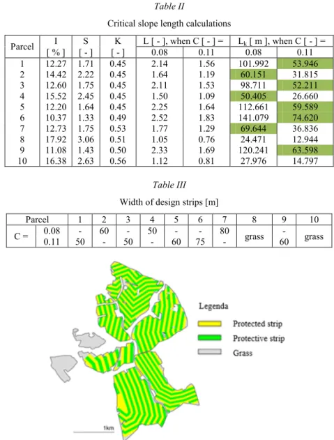
The mean value of a slope’s steepness (Fig. 7) was calculated from the DEM using GIS. From this map the S factor map (Fig. 7) was subsequently calculated. The results of the critical slope length are shown in Table II. Using these results, the contour strip cropping was designed as a valid soil control measure; the widths of both the protective and protected strips are shown in Table III. On parcels 1, 3, 5, 6, and 9, fodder crops will be rotated with crops with a C factor value of 0.11. On parcels 2, 4, and 7, fodder crops will be rotated with crops with a C factor value of 0.08. Since on parcel 8 and 10, the value of the slopes is higher than 15%, grassing is recommended. The design of the contour strip cropping is shown in Fig. 8.

Fig. 7. Slope steepness and S factor

Table II

Critical slope length calculations

Parcel I S K L [ - ], when C [ - ] = L_k [ m ], when C [ - ] =

[ % ] [ - ] [ - ] 0.08 0.11 0.08 0.11

1 12.27 1.71 0.45 2.14 1.56 101.992 53.946

2 14.42 2.22 0.45 1.64 1.19 60.151 31.815

3 12.60 1.75 0.45 2.11 1.53 98.711 52.211

4 15.52 2.45 0.45 1.50 1.09 50.405 26.660

5 12.20 1.64 0.45 2.25 1.64 112.661 59.589

6 10.37 1.33 0.49 2.52 1.83 141.079 74.620

7 12.73 1.75 0.53 1.77 1.29 69.644 36.836

8 17.92 3.06 0.51 1.05 0.76 24.471 12.944

9 11.08 1.43 0.50 2.33 1.69 120.241 63.598

10 16.38 2.63 0.56 1.12 0.81 27.976 14.797

Table III Width of design strips [m]

Parcel 1 2 3 4 5 6 7 8 9 10

C = 0.08 - 60 - 50 - - 80

grass -

grass

0.11 50 - 50 - 60 75 - 60

Fig. 8. Design of contour strip cropping 5.3. Design flow calculations

The aim of this estimation was to compare the design flow rate for the current land use of the river basin and the design flow rate for the land use of the river basin after the erosion measures were applied. The calculations were done using the CN number method. Using the orthophoto map, a land use map was created for Haluznikov Creek

basin. Based on this map and the soil type map, a map of the CN numbers was created (Fig. 9).

Fig. 9. Map of the land use and soil categories

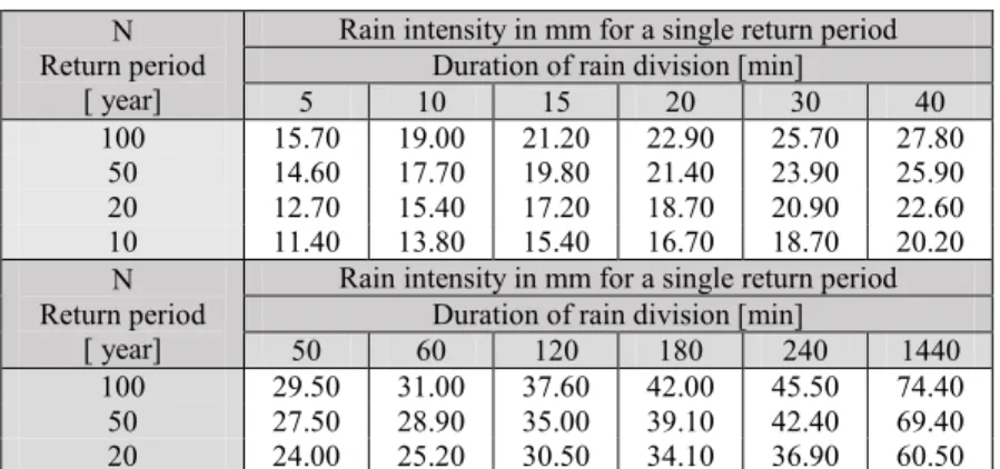
The design peak flow rate was calculated for return periods of 10, 20, 50 and 100 years from the values of the rain intensity as shown in Table IV. The rainfall intensity values that were input were divided from the one-day design values by a simple scaling method. The rainfall intensity values for the time concentration tkc = 72.77 min were determined by interpolation. Calculations were performed for three variants of land use:

in the first case the arable land is fallow; in the second case, the arable land is used for broad - row crops, and in the third case, the arable land is used for narrow - row crops.

The calculations of the design peak flow rates are shown in Table V and the reductions in design peak flows are shown in Table VI.

Table IV Rain intensity N

Return period [ year]

Rain intensity in mm for a single return period Duration of rain division [min]

5 10 15 20 30 40

100 15.70 19.00 21.20 22.90 25.70 27.80

50 14.60 17.70 19.80 21.40 23.90 25.90

20 12.70 15.40 17.20 18.70 20.90 22.60

10 11.40 13.80 15.40 16.70 18.70 20.20

N Return period

[ year]

Rain intensity in mm for a single return period Duration of rain division [min]

50 60 120 180 240 1440

100 29.50 31.00 37.60 42.00 45.50 74.40

50 27.50 28.90 35.00 39.10 42.40 69.40

20 24.00 25.20 30.50 34.10 36.90 60.50

Table V

Design peak flow comparison Arable land use Q₁₀

[m³.s^-1] Q₂₀ [m³.s^-1]

Q₅₀ [m³.^s-1]

Q₁₀₀ [m³.s^-1]

Fallow 10.71 12.89 16.11 18.05

Broad – row crops 8.99 10.89 13.70 15.42

Narrow – row crops 7.92 9.63 12.18 13.74

Fallow + fodder crops 9.18 11.11 13.97 15.72 Broad – row crops + fodder crops 8.39 10.18 12.85 14.48 Narrow – row crops + fodder crops 7.79 9.48 11.99 13.54

Table VI

Reduction in design peak flows

Arable land use Q₁₀ [ %] Q₂₀ [ %] Q₅₀ [ %] Q₁₀₀ [ %]

Fallow + fodder crops 14.3 13.8 13.3 12.9

Broad – row crops + fodder crops 6.7 6.5 6.2 6.1

Narrow – row crops + fodder

crops 1.6 1.5 1.5 1.4

6. Conclusion

The paper provides an overview of the data processing methodology for mean annual soil loss calculations and design peak flow calculations. The design peak flow calculations were done using the Curve Number method, because of its simplicity, and usefulness for ungauged watersheds.

The results of the soil loss calculations show that the area of interest is susceptible to erosion; for that reason, contour strip cropping was designed where protective strips with fodder crops will be rotated with protected strips with row crops.

The impact of the erosion measures was also assessed as flood protection measures.

With the contour strip cropping, the erosion was limited to an acceptable rate, and the peak flow rate was decreased.

In cases where the arable land is bare, the design peak flow Q10 will be reduced by 14% after applying soil loss measures, by 6.7% if the land is initially used for broad - row crops, and by 1.6% if the land is initially used for narrow - row crops. The design peak flow Q20 will be reduced by 13.8% if the arable land is initially bare, by 6.5% if the land is used for broad - row crops, and by 1.5% if the land is used for narrow - row crops. The design peak flow Q50 will be reduced by 13.3% if the arable land is initially bare, by 6.2% if the land is used for broad - row crops, and by 1.5% if the land is used for narrow - row crops. The design peak flow Q100 will be reduced by 12.9% if the arable land is initially bare, by 6.1% if the land is used for broad - row crops, and by 1.4% if the land is used for narrow - row crops. It follows that the measures will have the greatest impact on the design peak flow rates with a shorter return period.

Acknowledgments

This work was supported by the Slovak Research and Development Agency under Contract No. APVV-15-0425, APVV-15-0497, VEGA Agency 1/0710/15 and by the European Commission’s Seventh Framework Project RECARE, Contract No 603498.

The authors thank the agencies for their research support.

References

[1] Bosco C., de Rigo D., Dewitte O., Poesen J., Panagos P. Modeling soil erosion at European scale: towards harmonization and reproducibility, Nat. Hazards Earth Syst. Sci, Vol. 15, 2015, pp. 225–245.

[2] Panagos P., Borrelli P., Poesen J., Ballabio C., Lugato E., Meusburger K., Montanarella L., Alewell C. The new assessment of soil loss by water erosion in Europe, Environmental Science and Policy, Vol. 54, 2015, pp. 438–447.

[3] Kelčík S., Pindjaková T., Šoltész A. Assessment and design of the flood protection measures in the district of Levice (Slovakia), Pollack Periodica, Vol. 11, No. 1, 2016, pp. 35‒41.

[4] Shen Z. Y., Gong Y. W., Li Y. H., Hong Q., Xu L., Liu R. M, A comparison of WEPP and SWAT for modeling soil erosion of the Zhangjiachong watershed in the Three Gorges reservoir area, Agricultural Water Management, Vol. 96, No. 10, 2009, pp. 1435‒1442.

[5] De Vente J., Poesen J., Verstraeten G., Govers G., Vanmaercke M., Van Rompaey A., Arabkhedri M., Boix-Fayos C. Predicting soil erosion and sediment yield at regional scales:

where do we stand? Earth-Sci. Rev, 127, 2013 pp. 16–29.

[6] Merritt W. S., Lechter R. A., Jakemen A. J. A review of erosion and sediment transport models, Environmental Modelling and Software, Vol. 18, No. 8-9, 2003, pp. 761‒799.

[7] Wischmeier W. H., Smith D. D. Predicting rainfall erosion losses, A guide to conservation planning, Agriculture Handbook, No. 537, US Department of Agriculture, Washington, DC, 1978.

[8] Kinnell P. I. A. Event soil loss, runoff and the universal soil loss equation family of models:

a review, Journal of Hydrology, Vol. 385, No. 1-4, 2010, pp. 384‒397.

[9] Renard K. G., Foster G. R., Weesies G. A., McCool D. K., Yoder D. C. Predicting soil erosion by water: a guide to conservation planning with the Revised Universal Soil Loss Equation (RUSLE) Agriculture Handbook, No. 703, US Department of Agriculture, 2000.

[10] Výleta R., Celler M., Danačová M., Effect of erosion control on water erosion and sediment transport in the cadastre Sobotište, (in Slovak) Czech Journal of Civil Engineering, Vol. 2, 2016, pp. 162‒168.

[11] Výleta R., Danáčová M., Valent P. Analysis of change of retention capacity of a small water reservoir, IOP Conference Series: Earth and Environmental Science, Vol. 92, 2017, Paper 012075.

[12] Morgan R. P. C. Soil erosion and conservation, 3rd ed, Oxford, Blackwell Publishing, 2014.

[13] Panagos P., Borrelli P., Meusburger K., Alewell Ch., Lugato E., Montanarella L.

Estimating the soil erosion cover-management factor at the European scale, Land Use Policy, Vol. 48, 2015, pp. 38–50.

[14] Catholic University of Leuven in Belgium, 2016, https://www.kuleuven.be/english/, (last visted 30 Nov 2017).

[15] Desmet P. J. J., Govers G. A GIS-procedure for automatically calculating the USLE LS - factor on topographically complex landscape units, Journal of Soil and Water Conservation, Vol. 51, 1996, pp. 427‒433.

[16] Studvová Z., Danáčová M. Erosion and transport processes and their quantification by erosion models in terms of erosion control, vol. 3, 16th International Multidisciplinary Scientific GeoConference, Water Resources. Forest, Marine and Ocean Ecosystems, Albena, Bulgaria, 30 June - 6 July 2016, pp. 289‒296.

[17] Antal J. Soil protection and forest - technical melioration II, Instructions for exercises, (in Slovak), Príroda, Bratislava, 1989.

[18] Henige V., Bacúrik I. Protection and organization of the basin, (in Slovak) Slovak University of Technology, Faculty of Civil Engineering, Bratislava, 1998.

[19] Tepavčević B., Šijakov M., Šiđanin P. GIS technologies in urban planning and education, Pollack Periodica, Vol. 7: Supplement 1, 2012, pp. 185‒19.

[20] Real estate cadastral portal map, (in Slovak) Geodetic and Cartographic Institute, 2008, http://mapka.gku.sk/mapovyportal/, (last visted 30 March 2017).

[21] Heinige V., Hlavčová K., Bacúrik I. Protection and organization of the basin, Instructions for exercises, (in Slovak) Slovak University of Technology, Bratislava, 1995.