AN AGRO-ECOLOGICAL SIMULATION MODEL SYSTEM
M. LADÁNYI*–L. HORVÁTH –M. GAÁL – L. HUFNAGEL
*e-mail: mladanyi@kee.hu
Department of Mathematics and Informatics, Faculty of Horticultural Sciences, Szent István University, H-1118 Budapest, Villányi út 29–33, Hungary
(phone: +36-1-372-6261; fax: +36-1-466-9273)
(Received 15th April 2002; accepted 15th June 2003)
•
•
Abstract. In this paper five different models, as five modules of a complex agro-ecosystem are investigated. The water and nutrient flow in soil is simulated by the nutrient-in-soil model while the biomass change according to the seasonal weather aspects, the nutrient content of soil and the biotic interactions amongst the other terms of the food web are simulated by the food web population dynamical model that is constructed for a piece of homogeneous field. The food web model is based on the nutrient- in-soil model and on the activity function evaluator model that expresses the effect of temperature. The numbers of individuals in all phenological phases of the different populations are given by the phenology model. The food web model is extended to an inhomogeneous piece of field by the spatial extension model. Finally, as an additional module, an application of the above models for multivariate state-planes, is given. The modules built into the system are closely connected to each other as they utilize each other’s outputs, nevertheless, they work separately, too. Some case studies are analysed and a summarized outlook is given.
Keywords: food web, population dynamical model, activity function, spatio-temporal simulation model, multivariate state-planes
Introduction
The need to apply computer science and electronics in agricultural production for a targeted region has become increasingly urgent. By ’precision and sustainable agriculture’, we mean not only a new production method, but also a complex system that
integrates biological, technological and economic factors, and joins the natural circumstances flexibly.
This form of agriculture aims to optimize proficiency and environmental protection, by assessing together forecasts for risk, damages and profit.
In order to get to know better how the examined agro-ecosystem is functioning, we need correct simulation models of the complex food web system, as well as continuous monitoring of the processes [24, 31, 32, 37].
This simplified food web model accounts for seasonal weather aspects [74, 75], the nutrient content of soil and biotic interactions (Fig. 1). On the first level, K denotes the water and nutrient content of soil, as the input of the system. The input comes from a simplified nutrient-in-soil model [54] described below. Above the nutrient-in-soil term K, are cultivated plants, denoted by N, and two kinds of weed, denoted by G1 and G2, respectively. On the third level, monophagous M1 consumes the cultivated plant N, while monophagous M2 eats one of the weeds. P denotes a polyphagous pest which consumes the cultivated plant N, as well as weed G1. Additionally, there is a predator, denoted by P, that consumes pests M1, P and M2.
R
N
Ê
É
Ê
É
Ê
Ç
M P M
Ç
Ç
Ç
G G
Ç
K1 2
2 1
•
•
Figure 1. A food web model. The interactions amongst nutrient-in-soil (K), cultivated plant (N), weeds (G1 and G2), monophagous (M1 and M2) and polyphagous (P) pests, as well as predator (R). (The arrows run from the nutrient to the consumer.)
In this paper five different models, as five modules of a complex agro-ecosystem are investigated, furthermore, an extra module is constructed:
The water and nutrient flow in soil is simulated by the nutrient-in-soil model.
The biomass changes according to the seasonal weather aspects, the nutrient content of soil and the biotic interactions amongst the other terms of the food web, are simulated by the food web population dynamical model. The model is constructed specially for a piece of homogeneous field.
The activity function evaluator model expresses the effect of the daily average temperature on the activity of the individuals.
•
•
•
•
•
•
•
•
The numbers of individuals in all phenological phases of the different populations are given by the phenology model.
The food web model is extended for a piece of inhomogeneous field by the spatial extension model.
The last module gives an application of the above models for multivariate state- planes.
Although the modules built into the system are working separately, too, they are closely connected to each other, as they can utilize each other’s outputs:
The food web model is based on the activity function evaluator model and on the nutrient-in-soil model and it can immediately be followed by the phenology model.
The nutrient-in-soil model applies the outputs of the food web model as its own inputs.
The food web model and the spatial extension model can directly be linked.
The multivariate state-planes module is built on the results of the food web model completed with the phenology model and on the ones of the spatial extension model.
To simulate the interactions, a discrete difference equation system with daily scale is used. As in the literature, there are plenty of excellent models which describe certain parts of the processes quite exactly, our aim was to create a model that describes the whole interaction process, in order to be able to apply it also in cases when detailed data are missing and to extend it in cases when more complex data are available.
The pattern analysis and the investigation of spatio-temporal inhomogeneity of
sustainable agriculture. Additionally, it is important to elaborate the methodology of the information and data handling and the optimal decision making. Our aim is to go ahead in these problems. In former works the agro-ecosystem models (soil–plant–weather–
pest systems) and pattern analyses were operated separately. By a spatial extension of the agro-ecosystem model a space specific complex ecological model is obtained.
Some case studies are analysed and a summarized outlook, amongst others, of possible ways to develop and apply the models, is given.
Review of literature
After the first food web model was described by Shelford in 1913, the most popular early monography became Bird’s book from 1930 (In Jordán, [42]). Since that time, several theories have been appeared investigating the food web from several different points of view such as from energetical aspect [56], from population dynamical aspect [41], from stability, graph theory or information theory aspects [69, 70, 81, 82]. The structure of a food web and its interactions are characterized by Jordán [42, 44], while its reliability has been investigated by Jordán and Molnár, 1999; Jordán et al, 1999;
Jordán, 2000 [43, 45, 46]. In the past, there have been few papers published on food- web researches applied for Hungary.
Models have been constructed for ecosystems with food web simulations [65] that, nevertheless, are based on classical Lotka-Volterra interactions, ignoring either abiotic effects or phenological aspects. Crop–weed competition is investigated e.g. in Kropff and Laar [50] and a population–phenology simulator is applied by Mols [60, 61].
Agricultural modelling and empirical survey deal mainly with soil–plant–weather systems with different additional main points, such as climate change impact studies [10, 58], mineralisation and heat, water and nitrate transfer [18], soil heat and water dynamics
[27, 79], non-homogeneous cropped soil profile [47, 64], management impact [27, 77], environmental conditions [51, 62], water and nutrient dynamics in a plant [68] , fertilization [14], physiological and physical processes [8], water run-off and erosion in soil [49], phenology [48], planning and decision support [2, 3, 8], cropping systems [77]
and informatics [19, 20, 21]. Investigations of food web sytems are, however, not involved in the above studies. Comparisons of cropping systems can be found in Francaviglia and Marchetti [17] and in Giardini et al. [25]. A valuable review of methodologies to evaluate simulation models is given by Martorana and Bellocchi [59].
There have been published some recent papers on zoocoenological explorations of fresh-water patterns [4, 12, 13, 36, 81]. Investigations on agro-ecosystems can be found in Hufnagel et al. [32], in Ferenczy et al. [16] and in Nyilas et al. [64] for pest populations. Methodological questions of the ecosystem surveys are discussed e.g. in Hufnagel et al. [33, 34, 35] and in Gaál and Hufnagel [22, 23, 24], while the ones for agrosystem researches can be found in Harnos [28].
Results
Water and nutrient flow in soil
In order to minimize the difference between the optimal and the real results in agriculture, water and nutrient flow in soil have been observed yet from several aspects [5, 9, 83]. There was created a special, drastically simplified nutrient-in-soil model by
Erdélyi [15], with the special aim that it can be built into the food web population dynamical model to complete it with the most important abiotic effects.
The differential equation system of the nutrient-in-soil model consists of three equations: they follow the change of water, ionic nutrient and organic matter.
Water content of soil
As the plants can absorb ionic nutrient solution only, water content of soil plays as important role in vital processes as the ionic nutrient content of soil. The water content of soil is
reduced mainly by evaporation (of soil and plant), by take-up and water run-off;
•
• increased mainly by the precipitation and watering.
These factors are depending, amongst others, on temperature, global radiation, the relative water holding capacity and the growing rate of the plant, as well as the water holding capacity and the current water content of the soil. These effects are involved in our model, nevertheless, other properties of soil such as the amount of carbon dioxide, the effect of wind, etc. are ignored.
Water content of soil Vt+1 at the (t+1)th point of time can be calculated with the help of the water content of soil Vt at the tth point of time multiplied by an evaporation term
, a take-up term
Πt Ωt and, moreover, added to a precipitation – watering – and water run-off term Ψt:
1 t t t t.
t V
V+ = ⋅Π ⋅Ω +Ψ
Evaporation term is derived from the potential evapotranspiration formula due to Turc (in: Szász, [79]), that is given for the case water content is not limited and is corrected for the case water content does be limited which is the real case in Hungary.
Evaporation term Πt
Πt is depending on the daily temperature, the daily global radiation value and the current water content of soil. The more the water content is, the greater the rate of evaporation is, thus the less the evaporation term Πt is; 0 , and it is tending to 1 as the water content tends to zero.
<1 Π
< t
Take-up term is depending on the daily biomass growth and on the relative water holding capacity of the plant. The more the daily growth of the biomass is, the less take-up term is and with , take-up term
Ωt dBt
dBt
Ωt dBt →0 Ωt tends to 1.
Precipitation – watering – and water run-off term Ψt is depending on the daily precipitation, the daily amount of watering and the water holding capacity of soil.
Ionic nutrient and organic matter content of soil
Denote by the daily ionic nutrient solution content of soil that depends, of course, on the daily water content of soil V . Ionic nutrient solution content of soil at the (t+1)
Kt
t Kt+1
Kt
th point of time can be calculated by ionic nutrient solution content of soil at the tth point of time multiplied by a take-up term , an erosion term , and added to a decomposition term and an artificial fertilizer term :
It Et
Dt Kart,t
Take-up term (0< <1) is depending on the relative nutrient content of the plant derived from its need for ionic nutrient and on the daily biomass growth . It is obvious that the more the daily biomass growth is, the less take-up term is, and as the daily biomass growth dB tends to zero, take-up term goes to 1.
It It
dBt
It
dBt
t It
Erosion term (0< <1) expresses the fact that in case water is limited in soil, ionic nutrient solution is also limited by it, while in case water is unlimited, ionic nutrient solution is limited by ionic nutrient that is unable to be taken up by the plant.
Erosion term depends on the solubility of the different kinds of ionic nutrient. The greater amount of ionic nutrient is erosed the less amount of it is erosable, so erosion term tends to 1.
Et Et
Et
Et
Organic decomposition term at the tth point of time can be expressed by the formula
Dt
, )
1
( , ,
1 t biomt of t
t D D D
D+ = −ξ + +
where ξ<1 denotes the daily percent of the decomposed organic matter, denotes the amount of the developed organic matter in soil and denotes the amount of utilizable organic fertilizer added.
t
Dbiom, t
Dof,
The artificial fertilizer term is equal to the amount of the utilizable artificial fertilizer added.
t
Kart,
A food web seasonal population dynamical model
An agro-ecosystem is directed mainly by the interactions amongst the populations living in the agro-ecosystem together. Several indirect or hidden types of interactions that can not be expressed as different kinds of material flow such as competition, the indirect interactions that can be derived from the escape from or the defence against a common predator, as well as the so-called ’top down and bottom up regulations’ are involved in our food web population dynamical model. To simulate the interactions, a discrete difference equation system is used. The general equation of the web model is based on three elements: the first one is to express the activity of the individual depending on the temperature, the second one is to describe the effect of the quality and the quantity of nutrient of plants and/or pests and the third one is to display the effect of the predators. The model is based on the nutrient-in-soil model defined above.
To describe the interactions in the food web a discrete difference equation system with seven equations is used, each equation is for a certain element N, G1, G2, M1, M2, P, or R of the system at the (t+1)th point of time. The general form of the difference equation is
t X t X t X t
t X R F P
X +1 = ⋅ , ⋅ , ⋅ , , where
the current amount of the biomass of one of the populations N, G1, G2, M1, M2, P, or R at the (t+1)th and at the tth points of time are denoted by and , respectively;
+1
Xt Xt
•
the activity term of the individual X is denoted by and is depending on the daily average temperature
t
RX,
T;
•
t
FX, denotes the so-called nutrient term;
•
• PX,t denotes the so-called predation term.
In what follows the terms of the general equation are characterized.
Activity term RX,t
To forecast the time and the mass of the local appearance of pest generations, the so- called ’classical temperature-sum’ method is widely used, however, it is often unreliable and in these cases the errors can rush quite high. To avoid this, a parametric activity function that uses the data of the National Light-trap Network and the daily average temperature data as input, has been created by a special optimisation process by Révész [73]. Our model is based on the idea that was applied by Révész, namely, the agro- ecological process for each individual X is defined not by the temperature, itself, but by the so-called ’activity function’ that is a non-linear function of the daily average temperature T:
rX
(
( ) ( ))
,2 ) 1 (
: X X X fX
X T r T s T s T
r a = +
), exp(
) exp(
1 ))
( exp(
)) (
exp(
) 1 ( :
X X X
X X
X X
X X
X T s T a T b c T d a b c d
s − − +
−
− +
= − a
where aX, bX, cX, dX and fX are suitable constants relative to individual X.
Activity function expresses that the individuals do not develop under low temperature circumstances; while the temperature increases, the individuals develop at an increasingly rapid rate up to a certain point; at higher temperature as it is optimal for the individuals, the development is impeded peculiarly to the individuals’ sensitivity.
rX
Activity term RX is derived from the activity function rX by a linear transformation:
X X
X
X T A r T B
R : a ( )+ . The range of term RX is a narrow interval around number 1:
In the case the temperature is unfavourable, RX <1, the effect of the term is impedimental.
•
In the case the temperature is favourable, >1, the effect of the term is supporting.
RX
•
Term is continuous, monotonously increasing until the temperature is optimal and monotonously decreasing if the temperature is higher than it is optimal (Figs. 2 and 3).
RX
0,96 0,98 1,00 1,02 1,04 1,06 1,08
0 10 20 30
T e m p e r atu r e
R(T) for N, G1, G2 and P
0,92 0,94 0,96 0,98 1,00 1,02 1,04 1,06
1 36 71 106 141 176 211 246 281 316 351 Day
R_N
2 3 Figures 2–3. 2: Activity term of temperature (°C) for the cultivated plant N, weeds G1 and G2
and polyphagous P. 3: Activity term of day for cultivated plant N.
Nutrient term FX,t
Nutrient term is due to performance the following properties of the individuals in the model:
t
FX,
In the case nutrient is unlimitedly available (under fixed all other circumstances), the biomass of X is increasing at a maximal rate denoted by ΚX.
•
•
•
•
•
•
In the case nutrient is limited, the biomass of X is increasing more slowly, stagnating or decreasing.
In the case nutrient is just as much as needed, the amount of the biomass is nearly constant (FX ≈1).
In the case nutrient decreases excessively, the individual is going to die (FX →0).
In the case the individual is in competition with another consumer, the change of biomass is influenced by the amount of the biomass of the other consumer together with some weight parameters.
A polyphagous (P or R) consumes from the different populations in proportion to the amounts and the nutritive values of its nutrient-biomasses.
Term that satisfies all the properties above will be constructed step by step the following way. First, we give the proportion of the daily amount of total available nutrient reduced by the amount of necessary nutrient, and the amount of total available nutrient, more exactly the proportion
FX
XF
(-1)⋅(total available nutrient – necessary nutrient) total available nutrient
as follows:
ε +
−
−
− −
=
=
= K
G a G a N a G K
G
NF 1F 2F KN KG1 1 KG2 2 ,
ε
ε ε
+ +
⋅ +
⋅ +
− + + +
+ ⋅ + ⋅
−
−
−
=
1
1 1
1
1 1
1 1
1 1
1 1
1
G N
N G
P P
a P G G
N P P
a P M a N P
P G NP
NM
F ,
ε
ε +
⋅ +
⋅ +
− +
−
−
= N
G N
P P
a P M a N M
NP NM
F
1 1
1 1
1 1
1
,
ε +
− −
=
2
2 2
2
2 2
G
M a
M F G GM ,
+
+ + +
+
⋅ +
⋅ +
− + + +
⋅ +
⋅ +
− +
−
= ε
ε ε
2 1
2 1 2
1
1 1
1 1
1 1 1
1
M M P
M M P
R R
a R M P
P M
R R
a R M R
PR R
M F
+ + +
+
⋅ +
⋅ +
− +
− ε
ε
2 1
1 2
2 1
1 1
2
M M P
M P M
R R
a R M MR
.
Coefficients aXYdenote the weights of the narrows runnung from population X to Y, constant ε>0 is a tiny number due to avoid numerical errors during division. It is obvious, that XF >−1.
As the next step we introduce function
ν
= + x x f x
f 2
) 2 (
: a (x>−1)
that – substituting xby – satisfies all the properties above but the first one because its limit remains under ΚF
X
X even in case nutrient is unlimitedly available. Note that we choose ν >0 such that ν < lnΚX/ln2 holds.
Consider function
+
Κ
−
= 1, 1
1 2 max )
(
:x g x x
g a ν
0,99 0,995 1 1,005 1,01 1,015
-2 -1 0 1 2 3 4
x
Figure 4. Functions f (smooth line) and g (dotted line).
that is linear, continuous, strictly monotonously decreasing whenever and takes constant 1 if .
<0 x
≥0 x Function
) ( ) ( ) (
: F X F F F
X X F X g X f X
F a = ⋅
satisfies all the properties above including (i):
If −1< XF <0 that is to say, if nutrient is unlimitedly available:
•
ν
ν
⋅ +
+
− Κ
=
F F
F X F
X X F X X X
F 2
1 2 1 2
) (
: a .
If XF →−1 then FX →Κ, so substituting Κ by ΚX, we get that property (i) holds.
•
If XF ≥0, that is to say, if nutrient is just enough or short
•
ν
= +
F F
X F
X X F X X
F 2
) 2 (
: a
so, in the case nutrient is just enough (XF ≈0) thenFX ≈1, thus (iii) is satisfied.
Function FX is monotonously decreasing, thus (ii) holds.
•
•
•
•
In case , that is to say the individuals are starving, , as a consequence, they are going to die, so (iv) holds.
+∞
F →
X FX →0
Property (v) follows from the construction of , as we see that the decrease of the biomass of the nutrient-population is caused by the consumers-in- competition, together.
XF
Property (vi) follows from the construction of XF, again, with the brake effects 1
, 1 1 , 1
1 , 1 1 1
2 1 2
1+ N + P+M + M +M +
G and
1 1
1+ +M
P .
Predation term PX PX
•
Predation term satisfies the properties of the biomass-change as follows:
While the biomass of the consumer-population is increasing, the nutrient- population is decreasing at a slower and slower rate and, at the same time, the decreasing amount of the biomass of the nutrient-population is an impeding factor for the consumer-population. While the consumer-population is increasing slower, stagnating or decreasing, however, the amount of the biomass of the nutrient-population is going to stagnate or even to increase.
Consider the case of polyphagy. From the one nutrient-population’s aspect the effect of the other nutrient-population is, on the one hand, positive (while the other is being consumed, the one can escape), on the other hand, is negative (the other nutrient-population is making the consumer-population stronger by nourishing it).
•
The above effects of the interactions are quite complex. Our aim was to give the simplest model ever which describes the above properties as exactly as possible. It can be proved that terms
µ
ε
ε
⋅ + + +
⋅ +
⋅ + + +
=
N M M
a M G
N P P
a P P
NM NP
N
1 1
1
1 1 1
1 1 1
1
1
µ
ε
⋅ +
⋅ + + +
=
1 1 1 1
1
1
1 1
N G
P P
a P P
P G G
µ
ε
⋅ + + +
=
2 2 2
2
1 1
1
2 2 2
G M M
a M P
M G G
µ
ε
+
⋅ +
⋅ + + +
=
1 1 1 1
1
2 1
1 1
M P M
R R
a R P
R M M
µ
ε
+
⋅ +
⋅ + + +
=
1 1 1 1
1
1 2
2 2
M P M
R R
a R P
R M M
µ
ε
+
⋅ +
⋅ + + +
=
1 1 1 1
1
2
1 M
M P
R R
a R P
PR P
satisfy all the above properties where µ denotes a speed factor and ε >0 is a tiny number due to avoid numerical errors during division.
Multipliers
1 1
1 +
G , 1 1
+ N ,
1 1
2
1 +M +
M ,
1 1
2 +
+M
P and
1 1
1+ +M P
are to express the breaking effect in case more predators are in competition. The other poperties can be derived in a similar way we did before for nutrient term FX,t.
The connection of the nutrient-in-soil and the food web models Input data applied by the models can be devided into four groups:
Daily data such as precipitation, temperature, watering, global radiation, fertilization etc. These kinds of data have been available in Hungary for tens of years.
•
•
•
•
Constants related to the plant, soil, ionic nutrient or speeds of bioprocesses etc.
These kinds of data can be obtained by estimation or fitting.
Staring values like V , , etc. These kinds of data can be gained by e.g.
soil survey.
0, K0 D0
Other kinds of data such as the growth of biomass dBtdefined by
−
=
∑
−X s population all for
t t
t X X
dB : max ( 1),0 ,
organic matter Dbiom,t developed in soil defined by
−
=
∑
−X s population all for
t t t
biom X X
D , min ( 1), 0
etc. that are the outputs of the food web model and inputs of the nutrient-in-soil model, on the other hand, the available nutrient in soil that is the output of the nutrient-in-soil model and the input of the food web model. It is realized such that one step is taken by the nutrient-in-soil model, its output would be input into the food web model, one step is taken by which right after. Having the output of the food web model, the nutrient-in-soil model can be started again.
t
KX,
A case study for the population dynamical model.
Simulated results based on daily average temperature and precipitation data measured in 1980, Debrecen, Hungary
The models described above was tested with real temperature and precipitation data together with fictious but real proportional starting values K0,V0, S0, N0, G1,0, G2,0,M1,0, M2,0, P0, and R0 . The parameters of the activity terms as well as the coefficients aij and the constant ΚX were set such that they can demonstrate the different temperature sensitivity and some other properties of the different populations. In Fig. 3, it can be seen that for the different populations, the advantageous effect of activity term RX > 0 appears at different points of time in spring and, furthermore, that at about the 220th day of the year, there was a period with extremely high temperature and no precipitation, which was more or less impeding for every population.
Daily average temperature
-20,0 -10,0 0,0 10,0 20,0 30,0
1 33 65 97 129 161 193 225 257 289 321 353
Day
°C
N
0 1000 2000 3000 4000 5000
1 33 65 97 129 161 193 225 257 289 321 353 G1
0 500 1000 1500
1 33 65 97 129 161 193 225 257 289 321 353
G2
0 500 1000 1500 2000 2500
1 33 65 97 129 161 193 225 257 289 321 353 M1
0 500 1000 1500 2000 2500
1 33 65 97 129 161 193 225 257 289 321 353
M2
0 200 400 600 800 1000
1 33 65 97 129 161 193 225 257 289 321 353 P
0 500 1000 1500 2000 2500
1 33 65 97 129 161 193 225 257 289 321 353
R
0 500 1000 1500
1 33 65 97 129 161 193 225 257 289 321 353
Figure 5. Biomass change of cultivated plant N, weeds G1 and G2, monophagous M1 and M2 and polyphagous P, as well as predator R; a simulated result based on the daily average temperature measured in 1980, Debrecen, Hungary.
Compare temperature data with biomass data of the different populations in Fig. 5. (For the activity terms see Figs. 2 and 3.)
The biomass of cultivated plant N (from the last year) had been slowly decreasing till spring, then after having reached its optimal daily average temperature (in June) it was acceleratingly increasing. The growth came to a point of standstill at about the 220thday and after it reached its extended maximal rate, it was quickly decreasing.
Weed G1 prefers low temperature. It started to increase quite early, rather intensively.
In the middle of summer it was decreasing because of high temperature. After the average daily temparature fell below 15 °C, it increased again and started, again, to decrease quite late in autumn. In its graph, one can see the effect of fluctuating temperature in late autumn.
Weed G2 prefers higher temperature. It started to grow very quickly earlier than cultivated plant N. After the 250th day it was decreasing quite fast but the speed of decrease was lower and lower.
The activity term of monophagous M1 is similar to the one of its nutriant, thus their biomass graphs are similar, too, just with a short time shift.
Monophagous M2 consumes the weed that prefers higher temperature, though its optimal temperature is slightly lower. Therefore, it started to increase a bit later and slowlier than weed G1 and the same is for its biomass decrease.
Polyphagous P consumed from the early weed very few as it dislikes low temperature, however, it started to grow slowly. The decrease of the early weed left its mark on the graph of the pest. As the biomass of the cultivated plant started to increase quickly, the one of the polyphagous followed it and it started to decrease just after the cultivated plant’s biomass subsided.
Predator R can choose from three kinds of nutrient. It started to grow at about the 150th day at a stable rate, it reached its extended maximum with the marks of fluctuating temperature in late autumn/early winter which is followed by a very quick decrease.
Simulated results based on the daily average temperature and precipitation data measured in 1980-84, Debrecen, Hungary
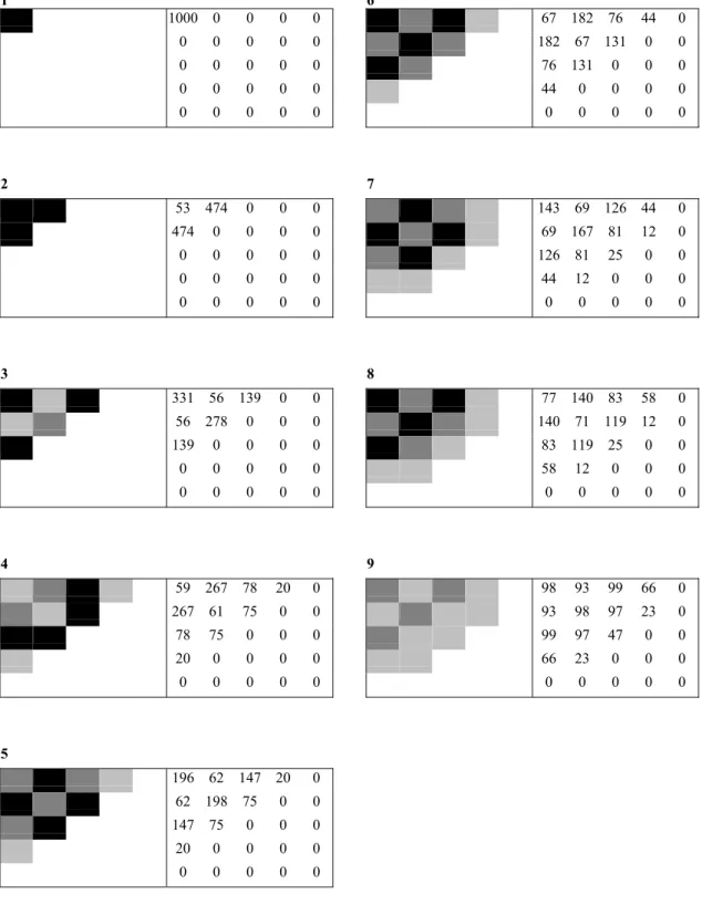
In Fig. 1, the seasonality relative to the populations can be seen well. While year 1983 was the most favourable for the cultivated plant N, yield in 1980 was quite poor (Fig. 6).
The effect of the mild winter in 1981–82 is considerable on the graph of the early weed G1.
Besides seasonality, it can be seen in the graph of the weed G2, which prefers warm weather, that the different conditions in different years imply graphs with different maximum, slope and convexity properties.
Notice the effect of a warmer (1981) and a cooler (1984) summer on monophagous G1 that prefers warm weather.
The graph of monophagous G2 that consumes the less sensitive weed seems to be the most stabile one.
Similarly to weed G1, polyphagous P prefers cool weather, thus years 1980–81 were more favourable than the ones after.
The graph of predator R can be said to be the less changeable.
Daily temperature 1980-84, Debrecen, Hungary
-20,0 -10,0 0,0 10,0 20,0 30,0 40,0
1 203 405 607 809 1011 1213 1415 1617 1819
N
0 500000 1000000 1500000 2000000 2500000
1 218 435 652 869 1086 1303 1520 1737 G1
0 50000 100000 150000 200000
1 213 425 637 849 1061 1273 1485 1697
G2
0 10000 20000 30000 40000 50000
1 207 413 619 825 1031 1237 1443 1649 M1
0 1000 2000 3000 4000
1 202 403 604 805 1006 1207 1408 1609 1810
M2
0 500 1000 1500 2000
1 202 403 604 805 1006 1207 1408 1609 1810 P
0 1000 2000 3000 4000
1 202 403 604 805 1006 1207 1408 1609 1810
R
0 2000 4000 6000 8000
1 192 383 574 765 956 1147 1338 1529 1720
Figure 6. Five-year (1980–84) simulation results of the food web model for each element of the web.
Phenology model
Applying the above models, the obvious question is how the number of individuals can be derived from a given amount of biomass. More exactly, if the phenological phases of the population, together with their biological properties, are known, how can one define the number of the individuals in the phases at a given point of time? The following model solves this problem.
Recall the idea mentioned in the section activity term was introduced, namely, that the agro-ecological process is not defined by temperature, itself, but by the so- called ’activity function’, since the effect of the same temperature on the individuals is very different in different phenological phases. Thus, instead of cumulative temperature, we introduce cumulative activity
t
RX,
Ph i X t
t i
Ph i X Ph
t t X
t R R SW
cum
X , X , ,
, , 0
0
⋅
=
∑
≥ =
with the help of which the entering dates of the phenological phases can be defined.
Cumulative activity cumulates the values of activity terms of individual X from a starting point of time relative to X (let us say ‘the first spring point of X’), in the case phase Ph holds, where Ph denotes one of E
Ph t t X
t R
cum
X ,
,
≥0
Ph t
RX,
t0,X
i (for the egg stateof the ith generation,
i = 1, 2, ... , gX), Lji (for the jth larva state of the ith generation, j = 1, 2, ... , lX) and Ii (for the imago state of the ith generation).
To express the phase Ph holds we introduce function for a population of X in a phenological phase Ph at a point of time t:
Ph t
SWX,
( )
( )
{ }
[ ] ( )
( )
{ }
[ ] [ { ( ) } ]
{ }
( )
>
>
−
− +
−
=
>
−
−
=
−
>
=
=
∏
∏
∏
>
−
>
>
11 ,
, , 1
,
11 ,
, ,
1 ,
1
,
0 1
*
* 1 , 1 , 0 , max
min 1 , 0 , max
min min
0 1
1 , 0 , max
min 1
0 0
:
1
1 1
1 1
L Ph and t
if SW
T CumR m
k m
L Ph and t
if SW T
CumR
E Ph if SW
E Ph and t
if
SW
L Ph
Ph t X
Ph X m Ph
t X Ph
Ph X X Ph
t X
L Ph
Ph t X L
X m t X E
Ph
Ph t X
Ph t
X ,
where
Ph X
Tm, denotes the minimum of cumulated activity of X that is necessary to enter phase Ph;
•
•
• Ph
t
mX, denotes the current average mass of an individual X in its state in phase Ph;
Ph
mX denotes the average mass of an individual X at entering phase Ph;
gX and denote the numbers of generations and larva phases related to X, respectively;
lX
•
Ph
kX is a proportion constant mPhX is multiplied by which in order to obtain the maximum mass of an individual X in phase Ph and, finally,
•
relation > for phases means „later phase than”.
•
•
•
•
•
•
Function equals to 1 if and only if the population of X has more than zero number of individuals in phase Ph at a given point of time t, and equals to 0, else. The change of the values of function
Ph t
SWX,
Ph t
SWX,
from 0 to 1 is caused by the fact cumulated activity has reached the minimum that is necessary for an individual X to enter phase Ph and/or by the one the mass of individual X has reached the maximum an individual in phase Ph can even have;
from 1 to 0 is caused by the fact the next phase has been entered.
With the help of function , a corrected food web biomass model can be created as follows:
Ph t
SWX,
. )
( )
( ) 1
)(
1
( ,
1 , 1
, 1
, ,
1 1
Ph t X Ph X g
i
I t X t
g
i
E t X t
g
i
I t X E
t X t
corr
t X SW SW W X SW I X SW LS
X =
∏
− i − i +∑
i +∑
i − χ=
=
= + +
The corrected food web biomass model above satisfies the following properties:
In winter there is no growth; in this case, function W of Xt expresses the biomass-waste caused by winter weather.
During the imago phase consumption is suspended; in this case, function I is the same as of the original food web biomass model, except term , which is now identically equal to 1.
+1
Xt FX
There is a loss in biomass at entering a new phase; function of denotes the amount of it, with characteristic function , that is equal to 1 if and only if t is the point of time phase Ph entered, and is equal to zero, else.
Ph
LSX Xt
Ph t X,
χ
It is obvious that there must be a point of time a phase is entered first, and, at the same time, there must be another one at which the process of metamorphosis is finished for the whole population. This means that function that ’switches’ on/off the phases has to be smoothed as follows:
Ph t
SWX,
1 1 1
, , ,
L t X E
t X E
t
X SW p
SSW = + ,
1 , ,
,
, = XPht*(1− XPht)+ XPht+
Ph t
X SW p p
SSW ,
where
1 1
1
1 1
1 ,
,
, ,0 ,1
1 2
max 1 min
1 L XLt
X L
X
L X L
t L X
t
X SW
MT MT
MT
p cumR ⋅
−
− −
= ,
Ph t Ph X
Ph X X Ph X
Ph Ph X X Ph
t Ph X
t
X SW
m c c
m c
p , m , ,0 ,1 ,
) 1 2 ( max 1 min
1 ⋅
−
⋅
− −
= for every Ph > L1.
This means that pPh is equal to zero until phase Ph is entered. In the case the
monotonously decreases from 1 to zero. At the point of time at which the whole process of metamorphosis is finished, pPhX,t becomes to be equal to, and also keeps to be, zero.
for
Ph
wX
X
⋅
χs
gX
It is easy to see that
.
, =1
∑
phases allPh t
SSWX
Finally, the numbers of individuals in all phases will be calculated as follows. Set out from an estimated starting value of the number of individuals at a starting point of time
in phase :
t0 E1
1 1 0
,0 E
X E t
t
X m
NoI = X ,
from which the numbers of individuals of later phases can be derived if Ph≠ Ei:
Ph t X s
t X Ph
t Ph X
X s t
t X Ph
t Ph X
X Ph t
t X Ph
t X Ph
t
X NoI SSW
m NoI X
p m NoI
NoI , ,01 , min , , 1 , min , , 1 (1 , ) ,
−
+
+
= − − χ − χ
1 0≤χXs,t ≤
where denotes a function to express the rate of starving of a population of X at a point of time t, calculated with the help of
the available amount of nutrient (denoted by NUXav,t), as well as
•
• the necessary amount of nutrient (denoted by NUXne,t) as follows:
=min ,1
, ,
, ne
t X av
t X t
X NU
NU .
Constant denotes the rate of maximum amount of weight that can be loosed without dying.
1 0<wPhX <
This formula is suitable to express the following properties of the populations:
The sum of the numbers of individuals does not increase in any phase except if
for .
Ei
Ph= i=1,2,...,
•
•
•
During the metamorphosis from a phase Ph into the next one, denoted by Ph+1, the number of individuals in phase Ph is decreasing tending to 0, while the number of individuals in phase Ph+1 is increasing.
The decrease of the biomass of X can be caused, on the one hand, by the fact that in case nutrient is short the individuals are losing their weights, and, on the other hand, by the one the population is consumed by another population. The number of individuals, in the first case, does not change, while, in the latter case, it is decreasing.
In case nutrient is shorter than it is necessary for the individuals even to keep being in existence, the number of individuals is decreasing because of starvation.
Note that the loss of biomass during the metamorphoses has been yet subtracted from the biomass of X.
The current average mass of an individual X in a phase Ph at a point of time t can be obtained as: