Large-scale Performance of a DSL-based Multi-block Structured-mesh Application for Direct Numerical Simulation

(1)

Large-scale Performance of a DSL-based Multi-block Structured-mesh Application for

Direct Numerical Simulation

G.R. Mudalige^a,∗, I.Z. Reguly^b, S.P. Jammy^c, C.T. Jacobs^d, M.B. Giles^e, N.D. Sandham^d

aDepartment of Computer Science, University of Warwick, UK

bFaculty of Information Technology and Bionics, Pázmány Péter Catholic University, Budapest, Hungary

cDepartment of Mechanical Engineering, SRM University, Amaravti, India

dAerodynamics and Flight Mechanics Group, Faculty of Engineering and the Environment, University of Southampton, Southampton, UK

eMathematical Institute, University of Oxford, UK

Abstract

SBLI (Shock-wave/Boundary-layer Interaction) is a large-scale Computational Fluid Dynamics(CFD) application, developed over 20 years at the University of Southampton and extensively used within the UK Turbulence Consortium. It is capable of performing Direct Numerical Simulations (DNS) or Large Eddy Simulation (LES) of shock-wave/boundary- layer interaction problems over highly detailed multi-block structured mesh geometries. SBLI presents major challenges in data organization and movement that need to be overcome for continued high performance on emerging massively parallel hardware platforms. In this paper we present research in achieving this goal through the OPS embedded domain- specific language. OPS targets the domain of multi-block structured mesh applications. It provides an API embedded in C/C++ and Fortran and makes use of automatic code generation and compilation to produce executables capable of running on a range of parallel hardware systems. The core functionality of SBLI is captured using a new framework called OpenSBLI which enables a developer to declare the partial differential equations using Einstein notation and then automatically carryout discretization and generation of OPS (C/C++) API code. OPS is then used to automatically generate a wide range of parallel implementations. Using this multi-layered abstractions approach we demonstrate how new opportunities for further optimizations can be gained, such as fine-tuning the computation intensity and reducing data movement and apply them automatically. Performance results demonstrate there is no performance loss due to the high-level development strategy with OPS and OpenSBLI, with performance matching or exceeding the hand-tuned original code on all CPU nodes tested. The data movement optimizations provide over 3×speedups on CPU nodes, while GPUs provide 5× speedups over the best performing CPU node. The OPS generated parallel code also demonstrates excellent scalability on nearly 100K cores on a Cray XC30 (ARCHER at EPCC) and on over 4K GPUs on a CrayXK7 (Titan at ORNL).

Keywords: DSLs, Multi-block Structured mesh applications, OPS, SBLI, Finite Difference Methods

1. Introduction

The exa-scale ambitions of the high performance computing (HPC) community, including major stakeholders in government, industry and academia, entail the development of parallel systems capable of performing an exa- FLOP (10¹⁸ floating-point operations per second) by the end of this decade [1,2]. The underpinning expectation is that performance improvements of applications could be maintained at historical rates by exploiting the increasing levels of parallelism of emerging devices. However, a key barrier that has become more and more significant is the difficulty in programming these systems. The hardware architectures have become complex where a highly skilled

∗Corresponding author

Email address: g.mudalige@warwick.ac.uk(G.R. Mudalige)

parallel programming know-how is required to fully exploit the potential of these devices. The issue has further been compounded by a rapidly changing hardware design space with a wide range of parallel architectures such as traditional x86 type CPUs with multiple cores, many-core accelerators (GPUs, Intel Xeon Phi), processors with large vector units, FPGAs, DSP[3] type processors and hetero- geneous processors. In most cases each architecture could be programmed using multiple parallel programming models while at the same time it is not at all clear which archi- tectural approach is likely to “win” in the long-term. It is unsustainable for domain scientists to re-write their applications for each new type of architecture or parallel system, as their code-base is typically large, usually compris- ing several millions of LoC. Furthermore, these code-bases most usually have taken decades to develop and validate to produce the required scientific output. Thus, developing

(2)

applications to be “future-proof” have become crucial for continued scientific delivery. A very closely desired feature is performance portability [4], where an application can be efficiently executed on a wide range of HPC architectures without significant manual modifications.

An emerging solution to future-proof applications and achieve performance portability is to separate the concerns of declaring the problem to be solved from its parallel implementation. The idea is to define the problem at a higher abstract level using domain specific constructs and then utilize automated code generation techniques to produce optimized parallel implementations. The technique then essentially allows scientists to maintain the “science”

source code without being tied to any platform specific implementation, acting as a base implementation of their model. At the same time, parallel computing experts then have the freedom to derive a parallel implementation using the best optimizations for a given parallel platform.

Translating the specification to parallel implementations is carried out by automated code generation techniques such as source-to-source translation and compilation. While this concept of abstraction is not new in computer science, its application to real-world high-performance computing code development has only been successfully attempted recently. In particular, domain specific languages (DSLs) have utilized this development strategy to great effect with a number of successful frameworks targeting several application domains [5,6, 7,8,9,10, 11, 12].

The underlying goals of this paper are to apply such high-level abstractions and code development for performance portability to large-scale production-grade codes, providing evidence of their utility in future-proofing HPC applications for the exa-scale. Here, we focus on the multi- block structured mesh SBLI (Shock-wave/Boundary-layer Interaction) application developed at the University of Southampton [13]. SBLI has been used extensively for projects within the Aerodynamics and Flight Mechanics group at Southampton as well as with DLR (The German Aerospace Center) [14], European Space Agency, Fluid Gravity Engineering, DSTL, to name a few, and is also representative of a number of codes within the UK Tur- bulence Consortium [15] and CCP12 for Computational Engineering[16]. At the University of Southampton, it is currently being used for Direct Numerical Simulation (DNS) or Large Eddy Simulations (LES) of shock-induced separation bubbles, receptivity and transition to turbulence and transonic flows. Its initial development was carried out over 20 years ago, but continues to be ac- tively maintained and optimized [17]. Simulations implemented in SBLI are typically direct numerical simulations [18] where the whole range of both spatial and tem- poral scales of turbulence is directly resolved by the computational mesh without utilizing any turbulence model.

In this case the number of mesh points increases rapidly with the Reynolds number.

Recently SBLI was re-engineered [19] to use the OPS [20] embedded domain specific language (EDSL).

OPS (Oxford Parallel library for Structured mesh solvers) is aimed at the development of parallel multi-block structured mesh applications and provides a domain-specific API embedded in C/C++/Fortran. It uses source-to- source translation to automatically parallelize applications written using this API. OPS is being used to parallelize a number of applications, including hydrodynamics [6], lat- tice Boltzmann codes [21] and CFD applications [22,23].

Currently supported parallel platforms include distributed memory clusters (using MPI), multi-core CPUs including Intel’s Xeon Phi many-core processors (using SIMD, OpenMP, MPI and OpenCL) and GPUs (using CUDA, OpenCL and OpenACC) including clusters of GPUs.

In this paper we present research that facilitated the re-engineering of SBLI to utilize OPS and charts the challenges and findings from converting a production- grade legacy application to ultimately execute on modern massively parallel many-core systems at peta-flop scales.

Specifically we make the following contributions:

1. We present the process of re-engineering SBLI to utilize OPS. The core functionality of SBLI is implemented using a new Python based open source framework called OpenSBLI [19], which enables a developer to define the problem to be solved at a higher level using Einstein notation. Multiple levels of automatic code-generation are then used to automatically carryout discretization of the problem and translating the higher-level “mathematical” description to a range of platform specific parallelizations. Our work demonstrates the clear advantages in developing maintainable, future-proof and performant applications through this high-level abstractions development strategy. To our knowledge this is the first production-grade multi-block application of its kind to be developed with a high-level abstraction DSL.

2. The multiple levels of abstraction exposes opportunities that can be exploited to increase parallelism and reduce data movement for improved performance. We present two such optimizations specifically aimed at improving the computation-communication balance in the application: (1) re-computing values within compute kernels without storing the values to temporary variables in RAM and (2) reducing memory accesses by tiling[24]. We generate code for OpenS- BLI that includes these optimizations and analyze its performance on a range of systems.

3. A representative application developed with OpenS- BLI is benchmarked on single node systems. These include systems with multi-core CPUs (Intel Broad- well, Intel Skylake, IBM Power 8) and many-core processors (NVIDIA P100, and V100 GPUs) parallelized with a range of parallel programming models including OpenMP, MPI, and CUDA. We com- pare the performance with that of the original hand- coded SBLI code while reporting achieved compute

(3)

and bandwidth performance on each system. Results demonstrate the versatility of OPS to produce highly performance portable applications.

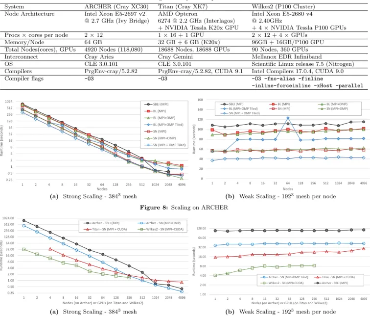
4. Finally, we present the performance of the OpenSBLI application (parallelized with OPS) comparing it to the performance of the original SBLI code on three large-scale systems, ARCHER at EPCC [25], Titan at ORNL [26] and Wilkes2 at the University of Cam- bridge [27] on nearly 100K CPU cores and over 4K GPUs. The OPS design choices and optimizations are explored with quantitative insights into their contributions with respect to performance on these systems.

Our work provides evidence into how DSLs and OPS in particular can be used to develop large-scale applications for peta-flop scale systems and demonstrates that in the same environment the performance is on par with the original. Furthermore, the new code is capable of out- performing the legacy applications with platform specific optimizations for modern multi-core and many-core/accel- erator systems.

The rest of the paper is organized as follows: In section2 we briefly introduce OPS including its API and code development strategy. Section3details the re-engineering of the SBLI application to utilize the OPS EDSL leading to the creation of the OpenSBLI framework. Section 4 presents performance from a representative multi-block application written using OpenSBLI and compares it to the legacy Fortran-based SBLI. Section5gives a brief overview of the state-of-the art with related work in this area. Section 6 concludes the paper.

2. The OPS Embedded DSL

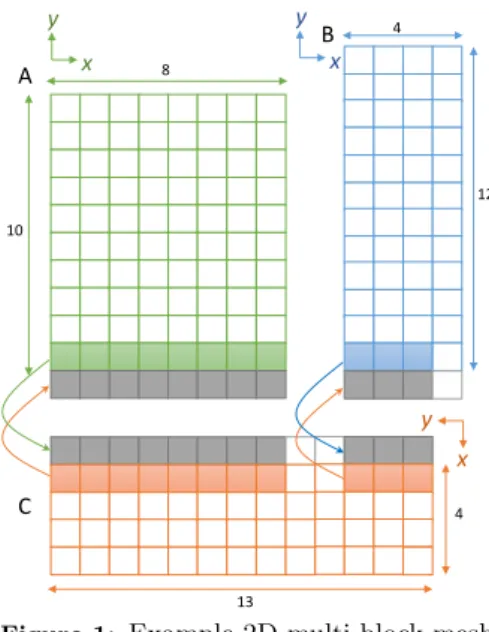
OPS (Oxford Parallel library for Structured-mesh solvers) [20] targets the domain of multi-block structured mesh applications. These applications can be viewed as computations over an unstructured collection of structured mesh blocks (see Figure 1). Within a structured mesh block, implicit connectivity between neighboring mesh elements (such as vertices, cells) are utilized. This is in contrast to unstructured meshes that require explicit connectivity between neighboring mesh elements via mappings.

As such, within a structured-mesh block, operations in- volve looping over a “rectangular” multi-dimensional set of mesh points using one or more “stencils” to access data.

While each block will be a structured mesh, a key characteristic of multi-block is the connectivity between blocks via block-halos.

OPS separates the above problem into five abstract parts. This enables a multi-block structured mesh application to be declared at a higher-level by a domain scientist. These parts consists of: (1) structured mesh blocks, (2) data defined on blocks, (3) stencils defining how data is accessed, (4) operations over blocks and (5) commu- nications between blocks. Declaring an application using

A

C

B

12

13

4 4

10

8

y x

x y

Figure 1: Example 2D multi-block mesh

these high-level domain specific constructs is facilitated by an API which appears to the developer as functions in a classical software library. OPS then uses source-to-source translation techniques to parse the API calls and generate different parallel implementations. These can then be linked against the appropriate parallel library enabling execution on different hardware platforms. The aim is to generate highly optimized platform specific code and link with equally efficient back-end libraries utilizing the best low-level features of a target architecture. The next section briefly illustrates the OPS API and code development with OPS.

2.1. OPS API

From the domain scientist’s point of view, using OPS is akin to programming a traditional single-threaded sequential application, which makes development and testing in- tuitive. Data and computations are defined at a high level, making the resulting code easy to read and maintain.

A typical multi-block scenario is illustrated in Figure 1. Here, three 2D blocks exist in affinity to each other.

The data set on the blocks share boundaries, where each boundary takes the form of a halo (called a block-halo) over which data is transfered¹. Furthermore in this case one of the blocks has a different orientation with respect to the other blocks. This multi-block mesh can be defined using the OPS API² as follows. We first define the blocks with its dimensionality and a name (string):

1 ops_block A = ops_decl_block(2,"A");

2 ops_block B = ops_decl_block(2,"B");

3 ops_block C = ops_decl_block(2,"C");

1The block halo is not to be confused with the typical distributed memory / MPI halos.

2We discuss and use the C/C++ API throughout this paper, but an equivalent Fortran API also exists

(4)

Next, data sets on each block are declared. Assume for this example that block A contains two data setsdat1and dat2 defined on it, while B and C each contain one data set (dat3 and dat4 respectively) defined on them. The two data sets defined on A each have a size of 10×8 and a block-halo of depth 1 at the start of their 2nd dimension (i.e. extending the data set in the negative y direction).

Similarly the data set on block B has a size of 12×4 and a block-halo of depth 1 at the start of its 2nd dimension (i.e.

extending the data set in the negative y direction). The data set on block C has a size of 13×4 and a block-halo of depth 1 at the start of its 1st dimension (i.e. extending the data set in the negative x direction).

4 int halo_neg1[] = {0,-1}; //negative block halo

5 int halo_pos1[] = {0,0}; //positive block halo

6 int size1[] = {10,8};

7 int base1[] = {0,0};

8 double* d1 = ... /* data in previously

9 allocated memory */

12 ops_dat dat1 = ops_decl_dat(A,1, size, base,

13 halo_pos1, halo_neg1, d1, "double", "dat1");

14 ops_dat dat2 = ops_decl_dat(A,1, size, base,

16

17 int halo_neg2[] = {0,-1};

18 int halo_pos2[] = {0,0};

19 int size2[] = {12,4};

20 int base2[] = {0,0};

23 ops_dat dat3 = ops_decl_dat(B,1, size, base,

25

26 int halo_neg3[] = {0,0};

27 int halo_pos3[] = {-1,0};

28 int size3[] = {13,4};

29 int base3[] = {0,0};

32 ops_dat dat4 = ops_decl_dat(C,1, size, base,

ops decl dat(...) declares a dataset on a specific block with a number of data values per data point (1 in this case for all threeops dats) and a size, together with parame- ters declaring the base index of the data set (i.e. the start index of the actual data), the sizes of the block halos for the data, the initial data values and strings denoting the type of the data and name of the ops dat. In this example arrays containing the relevant initial data (d1,d2and d3 of type double) are used in declaring ops dats. On the other hand, data can be read from HDF5 files directly using a slightly modified API call (ops decl dat hdf5).

Alternatively a null pointer can be passed as the data ar-

gument to ops decl dat, which will then be allocated as an empty data set internally by OPS so that it can be ini- tialized later within the application. Once a field’s data is declared via ops decl dat the ownership of the data is transferred from the user to OPS, where it is free to re-arrange the memory layout as is optimal for the final parallelization and execution hardware. Once ownership is handed to OPS, data may not be accessed directly, but can only be accessed via theops datopaque handles.

The above separation of data in OPS is driven by the principal assumption that the order in which elemental operations are applied to individual mesh points during a computation may not change the results, to within machine precision (OPS does not enforce bitwise repro- ducibility). The order-independence enables OPS to parallelize execution using a variety of programming techniques.

However it is not inconceivable to relax this restriction for implementing some order dependent algorithms within OPS, with the disadvantage being reduced flexibility for parallelizations. An example of such an order-dependent algorithm, currently being explored for implementation with OPS is the solution to a system of tridiagonal equations (see OPS repository on GitHub [28] feature/Tridiag- onal singlenode branch).

Once blocks and data on blocks are declared, the connectivity between blocks can be declared:

34 /* halo from C to A*/

35 int iter_CA[] = {1, 8}; // # elems in each dim

36 // starting index of from-block

37 int base_from[] = {0, 5};

38 // 1 = x-dim, 2 = y-dim

39 int axes_from[] = {1, 2};

40 // starting index of to-block

41 int base_to[] = {0,-1};

42 // -2 = negative y dim, 1 = x-dim

43 int axes_to[] = {-2,1};

44

45 ops_halo halo_CA = ops_decl_halo(dat3, dat1,

46 iter_CA, base_from, base_to,

47 axes_from, axes_to);

48

49 /* halo from A to C*/

50 int iter_AC[] = {8, 1};

51 int base_from[] = {0, 0};

52 int axes_from[] = {1,2};

53 int base_to[] = {-1,5};

54 int axes_to[] = {-2,1};

55 ops_halo halo_AC = ops_decl_halo(dat3, dat1,

56 iterAC, base_from, base_to,

57 axes_from, axes_to);

58

59 /*create a halo group*/

60 ops_halo grp[] = {halo_CA,halo_AC};

61 ops_halo_group G1 = ops_decl_halo_group(2,grp);

Currently, block-halo connectivity declaration is restricted

(5)

to a one-to-one matching between mesh points. In the above code listing, the connectivity between the blocks A and C (in Figure 1) are detailed. iter CA gives the number of elements in the block halos, i.e. the number of elements that will be copied over from C to A in each dimension. base from gives the starting index of the element on the source block that will be copied from and base to gives the starting index of the element on the destination block that will be copied to. axes from and axes todefines the orientation in which the elements will be copied from and to. For example, in the above code listing, if the x-dimension (represented by 1) is copied to the y-dimension (represented by 2) and y-dimension copied to the x-dimension, we define axes from[] = 1, 2 and axes to[] = -2,1. In the code listing the x-dimension is copied to the negative direction of the y-dimension, which is indicated by the-sign. Once the individual block halos have been defined, they can be combined into a group so that halo exchanges can be triggered for the whole group.

All the numerically intensive computations can be described as operations over the mesh points in each block.

Within an application code, this corresponds to loops over a given block, accessing data through a stencil, performing some calculations, then writing back (again through the stencils) to the data arrays. Consider the following typical 2D stencil computation:

1 int range[4] = {0, 8, 0, 10}; //iteration range

2

3 for (int j = range[2]; j <range[3]; j++) {

4 for (int i = range[0];i < range[1]; i++) {

5 d2[j][i] = d1[j][i] +

6 d1[j+1][i] + d1[j][i+1] +

7 d1[j-1][i] + d1[j][i-1];

8 }

9 }

An application developer can declare this loop using the OPS API as follows (lines 78-80), together with the “elemental” kernel function (lines 69-73):

62 /* Stencil declarations */

63 int st0[] = {0,0};

64 ops_stencil S0 = ops_decl_stencil(2,1,st0,"00");

65

66 int st1[] = {0,0, 0,1, 1,0, -1,0, 0,-1};

67 ops_stencil S1 = ops_decl_stencil(2,5,st1,"5P");

68 /* User kernel */

69 void calc(double *a, const double *b) {

70 b[OPS_ACC1(0,0)] = a[OPS_ACC0(0,0)] +

71 a[OPS_ACC0(0,1)] + a[OPS_ACC0(1,0)] +

72 a[OPS_ACC0(0,-1)] + a[OPS_ACC0(-1,0)];

73 }

74

75 /* OPS parallel loop */

76 int range[4] = {0,8,0,10};

77

78 ops_par_loop(calc, A, 2, range,

79 ops_arg_dat(dat2,S0,"double",OPS_WRITE),

80 ops_arg_dat(dat1,S1,"double",OPS_READ));

The elemental function is called a “user kernel” in OPS terminology to indicate that it represents a computation specified by the user (i.e. the domain scientist) to apply to each element (i.e. mesh point). By “outlining” the user kernel in this fashion, OPS allows the declaration of the problem to be separated from its parallel implementation. The ops par loop declares the structured block to be iterated over, its dimension, the iteration range and theops dats involved in the computation. OPS ACC0 and OPS ACC1are macros that will be resolved to the relevant array index to access the data stored in dat2 and dat1 respectively. The explicit declaration of the stencils (lines 63-67) will additionally allow for error checking of the user code. In this case the stencils consists of a single point referring to the current element and a 5-point stencil accessing the current element and its four nearest neighbors.

Further, more complicated stencils can be declared giving the relative position from the current(0,0) element.

TheOPS READindicates thatdat1will be read only. Simi- larly,OPS WRITE indicates thatdat2will only be accessed to write data to it. The actual parallel implementation of the loop is specific to the parallelization strategy involved.

OPS is free to implement this with any optimizations nec- essary to obtain maximum performance.

Theops arg dat(..) indicates an argument to the parallel loop that refers to an ops dat. A similar function ops arg gbl()enables users to indicate global reductions.

The related API call of interest concerns the declaration of global constants (ops decl const(..)). Global constants require special handling across different hardware platforms such as GPUs. As such, OPS allows users to indicate such constants at the application level, so that its implementation is tailored to each platform to gain best performance.

The final API call of note is the explicit call to com- municate between data declared over different blocks.

ops halo transfer(halos)triggers the exchange of halos between the listed datasets.

83 /* halo transfer over halo group G1 */

84 ops_halo_transfer(G1);

As mentioned before, for a givenops par loop, the order in which mesh points are executed in a block may be arbitrary. However, subsequent parallel loops over the same block respect data dependencies. For example the order in which loops over a given block appear in the code will enforce an execution order that OPS will not violate.

On the other hand, subsequent parallel loops over different blocks do not have a fixed order of execution and OPS is free to change this as appropriate. Only halo exchanges between blocks introduce a data dependency and therefore a prescribed order of execution between blocks. Further

(6)

details of the OPS API can be found in the user documen- tation [29], tutorial [30] and in [31,6].

2.2. Developing Applications with OPS

While input data structures are fixed, based on their description, OPS can apply transformations to tailor them to different hardware. OPS uses two fundamental techniques in combination to utilize different parallel programming environments and to organize execution and data movement. The first technique is to simply factor out common operations/functions for a given parallelization and indeed operations common to multiple parallelizations, and implement them within a classical software library. For example, the distributed memory, MPI-based message passing operations can be viewed as near-identical when used for passing messages between any type of node, be it a CPU based node, a GPU node or indeed other many-core nodes or nodes with hybrid processors. Such functions can therefore be readily implemented in a classical library, well optimized for the kind of message passing operations specifically found in multi-block structured mesh applications. Similarly, parallel file I/O operations such as using HDF5 to read in mesh data can also be factored out to a classical library.

The second technique is code generation or more specifically source-to-source translation, where it is used to produce specific parallelizations for theops par loopdeclara- tions. Thus for example, a parallel loop to be executed on a multi-core CPU needs to be a multi-threaded implementation and OPS needs to generate the code for a nested loop (based on the dimensionality of the loop) and also generate code to multi-thread the loop nest with OpenMP. The same loop, to be executed on a GPU will require the loop to be implemented for example using CUDA (i.e. OPS will need to generate CUDA code) including code to instruct the system to move data to and from the GPU.

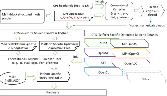
Figure2 gives an overview of the OPS work flow that a domain scientist will be using for developing a multi-block structured mesh application. The problem to be solved should be declared using the OPS API. During development, the application with API calls can be tested for accuracy by including a header file that provides a single- threaded CPU implementation of the parallel loops and the halo exchanges and compiling with a C++ compiler such as GNU’s g++ or Intel’s icpc. No code generation is required. This sequential developer version allows for the application’s scientific results to be inspected before code generation takes place. It also validates the OPS API calls and provides feedback on any errors, such as differences between declared stencils and the corresponding user kernels, differences between data types and/or mismatches between declared access types (OPS READ, OPS WRITE, OPS RW etc.) and how data is actually accessed in a kernel. All such feedback is intended to reduce the complexity of programming and simplify debugging.

Once the application developer is satisfied with the va- lidity of the results produced by the sequential application,

parallel code can be generated. At this stage, the API calls in the application are parsed by the OPS source-to-source translator which will produce parallelization-specific code (i.e OpenMP, CUDA, OpenCL, etc.) together with function/procedure calls to the relevant classical library. Thus, for example, to generate a version of the code that can run on a cluster of NVIDIA GPUs, OPS will produce CUDA code interspersed with calls to functions that implement MPI halo exchanges. The generated code can then be com- piled using a conventional compiler (e.g. gcc, icc, nvcc) and linked against the specific classical libraries to generate the final executable. As mentioned before, there is the option to read in the mesh data at runtime. The source-to-source code translator is written in Python and only needs to recognize OPS API calls; it does not need to parse the rest of the code. We have deliberately chosen to use Python and a simple source-to-source translation strategy to significantly simplify the complexity of the code generation tools and to ensure that the software technologies on which it is based have long-term support.

The use of Python makes the code generator easily modi- fiable allowing for it to even be maintained and extended by third-parties without relying on expertise of the original OPS developers. Furthermore, the code generated through OPS is itself human readable which helps with maintenance and development of new optimizations.

3. OpenSBLI : Automated Derivation of Finite- Difference Computations

OPS abstracts the parallel implementation of a multi-block structured-mesh problem. However, the problem needed to be declared at a level where loops over blocks and com- munications/transfers with block-halos are explicitly specified. As such, the problem needs to be posed as iterations over mesh points, i.e. loops and each loop needs to be declared as anops par loopstatement, together with code to set up the blocks, halos and data on blocks using the OPS API. A further increase in abstraction, one which is utilized in this research when re-engineering SBLI allows a scientist to declare a problem as a set of partial differential equations written in Einstein notation and then automatically generate C/C++ code with OPS API statements that performs the finite difference approximation to obtain a solution. The resulting DSL-based modeling framework called OpenSBLI is the subject of this section.

3.1. Re-Engineering SBLI to OpenSBLI

Legacy versions of SBLI, initially developed at the Uni- versity of Southampton over 20 years ago comprise static hand-written Fortran code, parallelized with MPI, that implements a fourth-order central differencing scheme and a low-storage, third or fourth-order Runge-Kutta time stepping routine. It is capable of solving the compress- ible Navier-Stokes equations coupled with various turbulence models (e.g. Large Eddy Simulation models), a TVD

(7)

OPS Source-to-Source Translator (Python) OPS Platform Specific Optimized Backend libraries

Conventional Compiler + Compiler Flags (e.g. Icc, nvcc, pgcc, ifort, gfortran)

Hardware

link

CUDA OpenMP

MPI OpenCL OPS Application

( C/C++/FORTRAN API)

Modified Platform Specific OPS Application

Platform Specific Optimized Application Files

Mesh (hdf5, ASCI)

Platform Specific Binary Executable Multi-block structured mesh

problem

MPI+CUDA MPI+OpenCL

OpenACC

Other … If correct numerical solution Conventional

Compiler (e.g. Icc, g++, ifort, gfortran) OPS header file (ops_seq.h)

include

Run on a single CPU

thread

Figure 2: The workflow for developing an application with OPS scheme to capture discontinuities in the flow and diag-

nostic routines. The code-base consists of over 64K LoC with multiple different versions of the application used for solving different numerical problems. The core of SBLI is the evaluation of central finite differences in the governing equations.

OpenSBLI, was developed from grounds-up as a replace- ment to SBLI, making use of code generation to produce the core functionality of the legacy code, but generating OPS API code which in turn enables us to target multiple hardware and parallel programming models [23]. As a result, new functionality is introduced where the finite difference problems that can be solved through OpenSBLI have become a superset of the legacy SBLI code.

To future-proof numerical methods based on finite difference formulations, OpenSBLI separates the numerical solution into two parts: (1) discretization of the governing equations, applying boundary conditions and advanc- ing the solution in time, known as the numerical method (mathematical manipulation), and (2) a computer code that performs the numerical method. OpenSBLI follows the principle that these two can be decoupled as the for- mer is purely mathematical in nature. Thus we can use symbolic mathematics by creating symbolic computations for the solution for the first part. The second part then involves converting the symbolic computations into a code based on the syntax of the desired programming language [23]. In our current work, this target language is C/C++

with the OPS API. A different DSL or a programming languages could also be targeted. Only the code-generation part of the framework should be rewritten. This capabil- ity gives rise to what we call “future-proofing numerical methods” where further decoupling the problem implementation from its declaration enables greater flexibility tailored to the context (e.g. numerical method and parallelization method). An additional outcome of this multi- layered strategy is that we are able to develop solutions

for finite difference problems beyond the original solvers in the legacy SBLI code-base. As demonstrated in this section one can easily add new equations, change the order of the numerical scheme as well as control the algorithm with relative ease.

OpenSBLI is written in Python and uses the symbolic Python library (SymPy) building blocks. The equation ex- pansion, numerical method discretization, boundary con- dition implementation and other mathematical manipulations are performed symbolically. To develop an application using OpenSBLI, the user describes the problem in a high-level Python script (which can be viewed as a problem configuration/setup file). This contains the partial differential equations to be solved along with the constituent relations, numerical schemes, boundary conditions and initial conditions. For example, consider the solution of the continuity equation in three dimensions with second order central difference scheme for spatial derivatives. The equations can be written in Einstein notation as:

∂ρ

∂t =−∂ρu_j

∂xj

(1) Here, ρ is density, uj is the velocity vector, xj are the coordinates and t is time. The components of the coordinates and velocity vector in three dimensions are given byx0, x1, x2andu0, u1, u2respectively. The key details of the high-level Python code to solve this equation is given below (for the full version see [23]).

1 mass = "Eq(Der(rho,t), - Der(rhou_j,x_j))"

2 ...

3 # Define coordinate direction symbol

4 coordinate = "x"

5 ndim = 3

6 # Create a problem

7 problem = Problem(mass, [], ndim, [],

8 coordinate, metrics=[None], [])

(8)

9 # expand the equations

10 expanded =

11 problem.get_expanded(problem.equations)

12

13 grid = Grid(ndim)

14 # Spatial Scheme

15 spatial_scheme = Central(2)

16 ...

17 # Perform the spatial discretization

18 discretise_s = SpatialDiscretisation(expanded,

19 [], grid, spatial_scheme)

20 ...

21 # Generate the code.

22 code = OPSC(grid, discretise_s, ....)

The continuity equation is written as strings in OpenSBLI (line 1). This equation is parsed into symbolic form and expanded depending on the number of dimensions of the problem (lines 5 – 11). OpenSBLI also facilitates break- ing up long equations into substitutions. Similarly, other equations to be solved along with any constituent relations are expanded. The numerical discretization of Equation1, requires a numerical grid (that is instantiated in line 13, with the number of points and grid spacing represented symbolically until later replaced with the inputs to a specific simulation). The discretization of the spatial terms in the equations, it requires the numerical scheme to be used. In the current example we are using a second order central finite-difference scheme. This is set by instantiat- ing theCentralclass, with desired order of accuracy as an argument. To change the order of accuracy, this argument needs to be changed. The rest of the script remains the same, showing the ease at which different codes can be generated. The spatial discretization is performed by calling theSpatialDiscretisationclass with the the expanded equations, constituent relations, the numerical grid and the spatial scheme as inputs. This class collects the spatial derivatives in the continuity equation (∂ρu_j/∂x_j) and applies the numerical method to create kernels. A kernel is a collection of equations that are to be evaluated over a specified range of the domain. A collection of kernels give the numerical solution. For example, the derivative

∂ρu0/∂x0 results in the following equations added to the kernel:

wk0 [0,0,0] = 1

2dx0(ρu0[1,0,0]−ρu0[−1,0,0]) (2) The array indexing used in OpenSBLI is the relative indexing approach, similar to the stencil indexing of OPS.

The creation of work arrays (e.g. wk0) or thread-/process- local variables can be controlled from a higher-level as we shall detail in Section3.2.1. Once all the kernels are generated for the spatial derivatives, these are ordered based on their dependencies and the original derivatives in the given equations are substituted with their work arrays.

The right hand side (RHS) of the equation is converted to:

RHS =−(wk0 [0,0,0] +wk1 [0,0,0] +wk2 [0,0,0]) (3) Similarly, computational kernels are created for tempo- ral discretization, boundary conditions, initialization, input/output, diagnostics etc. All the manipulations are symbolic and the framework, even at this stage of automatic generation, has no knowledge of the final programming language.

The final step is to convert all the symbolic kernels into a specific programming language. As described earlier we generate a compatible code using the OPS API. TheOPSC class (line 22) of OpenSBLI takes the symbolic kernels and convert them into OPS C/C++ code. Each kernel is written as anops par loopover the range of evaluation for that particular kernel. During this process, the type of access forops dat(read, write or read-write), number for OPS ACCand stencil access are derived from the equations defined for that kernel. The stencil accesses are created as a set to avoid repetitions.

To reduce computationally expensive divisions, the ra- tional constants, division by constants (likedx0) are evaluated to a constant variable at the start of the simulation.

The full list of optimizations performed are given in [22].

For easier debugging the entire algorithm used to generate the code can be written to a LaTeX file.

3.2. Computation vs. Data Movement Transformations When a problem is described at a high-level with OpenS- BLI and OPS, explicitly stating how and what data is accessed, it exposes opportunities that can be exploited to increase parallelism and reduce data movement. This allows the generated code to be tailored to different target hardware architectures. In this section we present two such transformations that significantly alters the underlying parallel implementation to achieve higher performance through balancing computation intensity vs. data movement.

3.2.1. Re-Computation of Values

With OpenSBLI, one can easily change the underlying algorithm to increase or decrease the amount of work arrays and or computational intensity of the algorithm. In this paper we generate two versions of the code (1) a baseline (referred to as BL) code and (2) a code requiring minimal storage (store none, SN). The BL algorithm follows the conventional approach frequently used in large-scale finite difference codes such as the original SBLI code. This contains subroutines orops par loop’s to evaluate the derivative of a function and store it to a temporary array. Due to ease of programming such an implementation, it is typically used when manually writing a finite-difference solver.

If a function is a multiple of two different variables (exam- plerho∗u0) then first the function is evaluated in a loop to a temporary array and then the derivative is evaluated to another temporary array using the subroutines. The BL algorithm uses 41 work arrays (same as SBLI) and 66

(9)

derivatives for the convective and viscous terms. Out of these 18 functions are a combination of two different variables (these are evaluated to a temporary variable first).

As such the algorithm has low computational intensity, but has significantly more data movement operations. In contrast to BL, the SN version does not store any derivatives to work arrays but the derivatives are stored to local variables and are used to evaluate the right hand side of the equations. If we consider the discretization of the continuity equation (Equation1), the RHS is evaluated as:

var0 = 1

2dx0(ρu0[1,0,0]−ρu0[−1,0,0]) (4) var1 = 1

2dx1(ρu1[0,1,0]−ρu1[0,−1,0]) (5) var2 = 1

2dx2(ρu2[0,0,1]−ρu2[0,0,−1]) (6) RHS=−(var0 +var1 +var2) (7) If a derivative has combination of two different variables or for mixed derivatives (∂u0/∂(x0x1)), the function or the inner derivative ∂u0/∂x0 is recomputed across the stencil. This increases the computational intensity of the algorithm, while reducing memory accesses. Such an algorithm is generated by setting the store derivatives attribute of the grid class to False. In addition to BL and SN, the ease at which such modifications can be performed is explained in detail by generating several other variations of the solver in [22].

3.2.2. Tiling

Most computational stages in OpenSBLI, and generally in structured-mesh CFD are bound by how fast the architecture can move data between the processor and main memory. As described above, one way of addressing this is via algorithmic optimizations, but it is also possible to improve data re-use by changing the scheduling of operations. For example, if two subsequent parallel loops access some of the same data, this data (due to its size) will not stay in cache between accesses. Therefore the second loop has to read it again from RAM. However, by only scheduling some of the iterations in the first loop, accessing just a subset of the entire dataset, and then, accounting for dependencies, scheduling the appropriate iterations in the second loop, we can exploit data re-use between these two loops.

This implements a type of cross-loop scheduling, which in this use case we call cache-blocking tiling. Program- ming such an optimization manually is tedious and virtu- ally impossible for large-scale codes. Traditional compilers and Polyhedral compilers [32, 33,34, 35,36, 37,38] have been targeting this problem for many years, yet they are not applicable to problems of this size. Therefore in OPS we have implemented a feature that determines the cross- loop dependencies and constructs execution schedules at runtime [24]. On top of achieving better cache locality, the algorithm also improves distributed-memory commu- nications; by determining inter-process data dependencies

for a number of computational steps ahead of time, it can group MPI messages together and exchange more data but less frequently. Additionally, it can avoid communicating halos for working arrays altogether, by redundantly computing around the process boundaries.

Tiling in OPS relies on delaying the execution of parallel loops, and queuing up a number of them to analyze together. Execution has to be triggered when some data has to be returned to user space. In OpenSBLI we can analyze a large number of loops together, because data is only returned to the user at the end of the simulation. Af- ter some experimentation we found that the optimum is to analyze and tile over all the loops in a single time step.

4. Performance

Having re-engineered SBLI to OpenSBLI, we validated the results from the new code to ascertain whether the correct scientific output is produced. Validation consisted of running OpenSBLI on known problems, comparing its results to the legacy SBLI application solving the same problem.

The correctness of different algorithms on CPUs were previously reported in [22]. In the present work, the min, max difference between the algorithms for all the conser- vative variables were found to be less than 10⁻¹² on each architecture, and the difference between the runs on CPU, and GPU are found to be less than 10⁻¹² for the number of iterations and the optimization options considered here.

After establishing accuracy, the remaining open ques- tion is whether the time and effort spent in re-engineering SBLI to utilize OPS, producing OpenSBLI was justified in terms of performance. The key questions are (1) whether the utilization of OPS through OpenSBLI affected (improved/degraded) the performance compared to SBLI (2) what new capabilities can be enabled through OPS that improve performance, (3) whether further performance gains are achievable with modern multi-core/many-core hardware, (4) what quantitative and qualitative performance gains result in computation vs. data movement transformations on different parallel platforms and (5) whether OpenSBLI scales well, considering large-scale systems (with node architectures of pre-exascale and upcom- ing exascale designs) and problem sizes of interest in the target scientific domains.

We begin by determining whether using a high-level approach such as OpenSBLI and OPS is in any way detri- mental to performance when compared to the hand-coded original; it is obviously important to be able to perform a like-for-like comparison and demonstrate that the OPS version can indeed match the performance of the original under identical circumstances. We first explore the single node performance in Section4.1 followed by performance on a number of large-scale distributed memory systems in Section4.2.

As mentioned before, a number of known problems were used for validating OpenSBLI [23, 39, 40]. One of them is the 3D Taylor-Green Vortex problem [41,42,43], which

(10)

Table 1: Single node Benchmark systems specifications

System Kos Scyrus Saffron

Node Intel Xeon Intel Xeon POWER 8E

Architecture E5-2660 v4 @ 2.0GHz (Broadwell) Silver 4116 CPU @ 2.10GHz 8247-42L @ 2.06 GHz + 1×NVIDIA Tesla V100 GPU (Skylake)

+ 3×NVIDIA Tesla P100 GPUs

Procs×cores 2×14 (2 SMT/core) 2×12 (2 SMT/core) 2×10 (8 SMT/core)

Memory 132 GB 96 GB 268 GB

+ 16GB (P100) and 16GB (V100)

O/S Debian 4.9.51 Debian 4.9.82 Ubuntu 16.04 LTS

Table 2: Compilers and Compiler Flags

Compiler Version Compiler Flags

Intel Compilers 18.0.2 Broadwell and Skylake : -O3 -fno-alias -finline -inline-forceinline icc, icpcandifort -fp-model strict -fp-model source -prec-div -prec-sqrt -xHost -parallel

nvcc CUDA 9.1.85 -O3 -restrict --fmad false

P100 : -gencode arch=compute 60,code=sm 60 V100 : -gencode arch=compute 70,code=sm 70

IBM XL C/C++ V13.1.7 (Beta 2) -O5 -qmaxmem=-1 -qnoxlcompatmacros -qarch=pwr8 -qtune=pwr8

xlc, xlc++andxlf for Linux -qhot -qxflag=nrcptpo -qinline=level=10 -Wx,-nvvm-compile-options=-ftz=1 -Wx, -nvvm-compile-options=-prec-div=0 -Wx,-nvvm-compile-options=-prec-sqrt=0

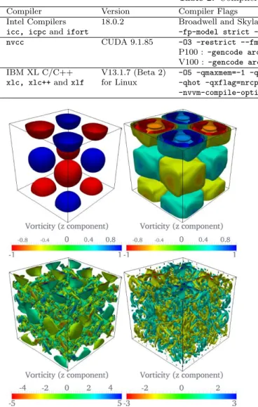
Figure 3: Non-dimensional vorticity iso-contours from the Taylor-Green vortex problem (256³ mesh). Top left to bottom

right: non-dimensional time t = 0, 2.5, 10, 20. [23]

we use in this section to benchmark and explore performance. This problem considers the evolution of a vortex system, starting from the initial stages of roll-up, stretch- ing and vortex-vortex interaction, all the way to vortex break-down and transition to turbulence. No turbulence is artificially induced/generated, such that all the energy is dissipated by the small-scale structures with the com- pressible fluid eventually coming to rest. The numerical method must be capable of accurately representing each of these physical processes/stages [23]. Figure3presents a visualization of the z-component of vorticity in the Taylor-

Green vortex test case with a 256³mesh points, at various non-dimensional times.

4.1. Single Node Performance

Table1provides brief specifications of the single node systems used in our initial performance analysis. The first system, Kos is a single node system consisting of two Intel Xeon Broadwell processors together with multiple NVIDIA GPUs, 1 × Tesla V100 and 3 × Tesla P100.

Each Intel processor consists of 14 cores each configured with 2 hyper-threads (SMT). The second system, Scyrus consists of two Intel Skylake processors, each consisting of 12 cores. Again, each core is configured to have 2 hyper- threads. The final system, Saffron, is an IBM POWER8 processor system. It consists of two POWER8 processors, each with 10 cores. Each core is configured to run up to 8 hyper-threads. The compilers and flags used to build SBLI and OpenSBLI applications and OPS are detailed in Table 2. We believe these three single node systems, including the GPUs in them, adequately represent current multi-core and many-core node architectures used in large-scale machines. Performance on these systems provides initial insights into the key questions posed above.

For the remainder of the paper we focus on the performance of the main time-marching loop without considering time spent in file I/O. In production runs it is common to use file I/O for regular checkpointing. A previous paper [44] with OPS demonstrates how high-level abstractions improves the performance of checkpointing. Of particular note is one of the checkpointing modes in OPS that enables a separate thread of execution to save data to disk as a non-blocking call that executes asynchronously. As such there is minimal impact to performance with checkpointing. In the experiments for this paper we do not do any checkpointing as we only focus on time to solution.

4.1.1. Runtime Performance

Figure4(a) and (b) presents the runtime (100 iterations) of the baseline Taylor-Green Vortex application, BL and

(11)

85.80 108.80

32.40

12.00 8.05

65.64 66.35 72.51 94.92

83.16 70.86

33.02 46.79

62.31

0.00 20.00 40.00 60.00 80.00 100.00 120.00

SBLI on CPU Nodes P100 V100 SkyLake Broadwell POWER8

MPI + OMP + Tiled CUDA MPI + OMP MPI

(a) SBLI vs OpenSBLI-BL

85.80 108.80

32.4

4.36 2.93

28.98 29.35 30.19 32.18 31.15 30.24 15.67

35.08 24.18

0.00 20.00 40.00 60.00 80.00 100.00 120.00

(b) SBLI vs OpenSBLI-SN Figure 4: Taylor-Green Vortex, Single node runtimes (seconds) - 192³Mesh

207.60 264.30

84.80

30.57 19.85

161.00169.15 155.53

222.20 203.47

158.17

77.92 106.75

138.79

0.00 50.00 100.00 150.00 200.00 250.00 300.00

(a) SBLI vs OpenSBLI-BL

207.60 264.30

84.80

10.91 7.12 81.38 82.19

69.46 81.10 80.74 59.78

36.26 85.71

63.08

0.00 50.00 100.00 150.00 200.00 250.00 300.00

(b) SBLI vs OpenSBLI-SN Figure 5: Taylor-Green Vortex, Single node runtimes (seconds) - 260³Mesh

the SN version of the application solving a mesh of size 192³ on the single node benchmark systems. Recall that the SN (Store None) version of the code, has a higher computational intensity, where instead of evaluating the derivatives and storing them on to work arrays, the OpenS- BLI code generation process directly replaces the derivatives by their respective finite difference formulas such that they are recomputed every time. The figures present all parallel versions generated through OPS that can execute on each of the benchmark systems in Table 1. For comparison, the first three bars of the graph indicate the runtime of the same problem (and problem size) solved by the original SBLI application on the Skylake, Broadwell and POWER8 nodes respectively. MPI distributed memory parallelism is the only parallel version supported by SBLI.

We see that the baseline Taylor-Green Vortex version, BL implemented with OpenSBLI matches the same application implemented using the legacy SBLI code for this problem size (see Figure4(a)). The MPI parallel version of BL is actually 30% faster on the Skylake and 15% faster on the Broadwell systems than its SBLI counterpart. On the IBM POWER8, BL gives almost the same runtime as SBLI (less than 2% difference). This result gives us an initial indication that the high-level abstraction and code generation has not resulted in any degradation in performance compared to the original hand-tuned version. Other parallelizations on the Broadwell node give further performance improvements (4×MPI+12×OMP+Tiling giving about 30% speedups), while the MPI only version of BL gives the best performance on the Skylake and POWER8.

Considering the performance of BL across systems, the best CPU performance is given by the POWER8 system (running 80× MPI procs) with nearly 2× speedup compared to the two-socket Skylake system (24× MPI) and over 2× speedup compared to the two-socket Broadwell system (4× MPI+14×OMP+Tiled). However, the best overall performance is achieved on the single GPUs using CUDA, with close to 4×speedup over the best CPU performance (POWER8, 80×MPI) on the V100 GPU. The V100’s speedup over the original SBLI code is also about 4×.

Considering the SN version of the application (Fig- ure4(b)), we see close to 3×speedup over SBLI on Skylake (48×MPI), 3.3× speedup on Broadwell (56× MPI) and 2× speedup on POWER8 (80×MPI). The MPI-only SN version also provides over 2×speedup over the MPI-only BL version on the Skylake node and nearly 3× over the MPI only BL version on the Broadwell node. Similarly the SN MPI runtime given by the POWER8 is just over 2×

faster than its BL MPI runtime. As such it is evident that optimizing for reducing memory accesses / communica- tions have played a considerable role in improving the performance of the application. The performance of the SN version across systems show that now there are less performance differences between CPU systems. GPUs still give the best runtimes with over 5×speedup given by SN on the V100 GPU over the best performing CPU (POWER8, 80×MPI).

Results from benchmarking the same problem on a

(12)

43.76 68.54

36.94

10.56 7.08

33.48 44.64

37.64

3.83 2.58 14.78

19.05 17.86

0.00 10.00 20.00 30.00 40.00 50.00 60.00 70.00 80.00 90.00

Energy Consumption (kJ)

Skylake (630W) Broadwell (510W) Power8 (1140W) P100 (880W) V100 (880W)

SBLI on CPU OpenSBLI - BL OpenSBLI - SN

(a) 192³

105.88 166.51

96.67

26.90 17.47

79.32 99.65

88.83

9.60 6.26

35.42 37.66 41.33

0.00 20.00 40.00 60.00 80.00 100.00 120.00 140.00 160.00 180.00

Energy Consumption (kJ)

Skylake (630W) Broadwell (510W) Power8 (1140W) P100 (880W) V100 (880W)

SBLI on CPU OpenSBLI - BL OpenSBLI - SN

(b) 260³ Figure 6: Single node energy consumption (kJ)

larger problem size of 260³is given in Figure5(a) and (b).

In this case, the problem size was chosen such that it max- imizes the global memory used on both the P100 and V100 GPUs. Any larger mesh, we found could not be solved by a single GPU with OpenSBLI-BL (the SN version uses less memory). Again we see most of the performance trends from the smaller problem size occurring for the larger problem size. The performance differences between SBLI and the MPI versions of BL on Skylake and Broadwell are now 28% and 18% respectively. On the POWER8, BL performs with a 8% speedup over SBLI. The best BL version on the CPU systems was again on the POWER8 (80×MPI). We also see that there is again a notable benefit of tiling on the Broadwell system with about 30% improvement over MPI+OpenMP. Some minor improvements with tiling is also observable on Skylake. However, as before the best overall runtime is given by the V100 GPU. This is close to 4×speedup over BL and 4.2×over SBLI on the POWER8 system (80×MPI).

Considering the SN version on the 260³problem size in Figure 5(b), we see similar performance trends as before.

The V100 GPU, is now giving over 5×speedup compared to the best runtime on a CPU system, in this case given by the POWER8 (80×MPI) node.

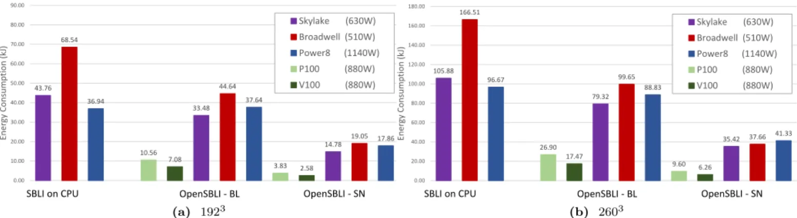
4.1.2. Power and Energy Consumption

While the runtime performance shows GPUs giving significant speedups over CPUs, it is always difficult to judge performance solely on time to solution. This is particularly true due to the fact that in order to run applications on a GPU, it currently needs to be hosted on a system with a CPU. All the GPU systems we present results for has this characteristic. A fairer cost metric could be the energy consumption of a simulation depending on the hardware.

Such a measure could be obtained by estimating the power consumed by the single node system, multiplying it by the runtime of the simulation on that system.

We use the thermal design power (TDP) to estimate the power consumed by each processor. A single Intel Xeon Broadwell CPU has a TDP of 105 Watts[45]. The two socket system used in these experiments will therefore consume upto 210 Watts. We triple this value (630

Watts) to account for the power draw of the whole node, due to memory, disk, networking etc. A similar figure of 510 Watts is calculated for the dual socket Skylake system [46] and 1140 Watts for the dual socket POWER8 [47]

system. Both P100 and V100 GPUs each has a TDP of 250 Watts [48, 49]. Given that the runtime figures only consider 1 GPU executing the application we assume that the power consumption will be equivalent to the TDP of a single GPU plus three times the TDP of the dual socket Intel Broadwell CPUs that hosts it. This gives a total of 880 Watts per GPU. These estimates appear to be ac- ceptable compared to the single-node power consumption figures of the three cluster systems we use in Section4.2.

Figure 6 details the energy consumed during the best runtimes on each architecture for SBLI and OpenSBLI’s BL and SN versions. Energy consumption for both problem sizes give similar CPU vs GPU trends. While both the P100 and V100 has a larger power-draw than the Intel CPUs, due to the higher runtime speedups the GPUs ex- hibit superior energy efficiency per execution. For the best performing SN version, on the 192³problem, the P100 and V100 are over 3×to just over 7×more energy efficient than any of the CPU runs. A similar energy efficiency speedup can be observed for the 260³ problem. The key insight, as we have previously observed is that for the above OpenS- BLI application versions [50] and similar mesh based traditional HPC applications [5] the most energy efficient ex- ecutions are almost always achieved by the systems giving the fastest runtime.

4.1.3. Computation and Bandwidth Performance

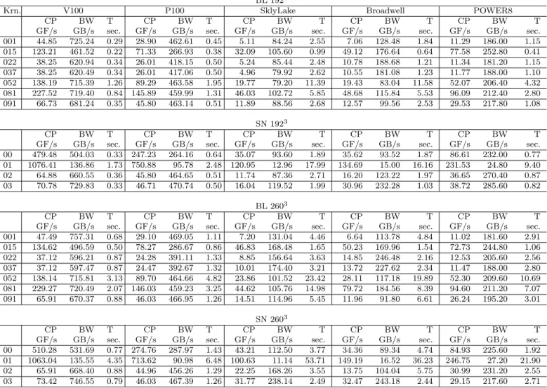
Investigating the achieved computation performance, in terms of achieved Flops/s and the achieved bandwidth on each system provides further insights into the behavior of the application, especially given the significant performance difference of the BL and SN versions, and given the memory access optimizations in SN. Table3 details these achieved performance results for the most time consuming kernels in the BL and SN versions of the applications.

Seven kernels are selected for BL of which three (001,022,037) are for the evaluation of multiple functions as described in Section3.2.1, one each for the evaluation of