Computer Physics Communications

(1)

Contents lists available atScienceDirect

Computer Physics Communications

journal homepage:www.elsevier.com/locate/cpc

Efficient GPU implementation of the Particle-in-Cell/Monte-Carlo collisions method for 1D simulation of low-pressure capacitively coupled plasmas

^✩

Zoltan Juhasz

^a^,^∗

, Ján Ďurian

^b

, Aranka Derzsi

^c

, Štefan Matejčík

^b

, Zoltán Donkó

^c

, Peter Hartmann

^c

aDepartment of Electrical Engineering and Information Systems, University of Pannonia, Egyetem u. 10, Veszprem, 8200, Hungary

bDepartment of Experimental Physics, Faculty of Mathematics, Physics and Informatics, Comenius University in Bratislava, Mlynská Dolina F2, 842 48 Bratislava, Slovak Republic

cWigner Research Centre for Physics, Konkoly-Thege M. str. 29-33, Budapest, 1121, Hungary

a r t i c l e i n f o

Article history:

Received 2 October 2020

Received in revised form 11 January 2021 Accepted 16 February 2021

Available online 26 February 2021

Keywords:

Collisional plasma simulation Particle-in-Cell method GPU

a b s t r a c t

In this paper, we describe an efficient, massively parallel GPU implementation strategy for speeding up one-dimensional electrostatic plasma simulations based on the Particle-in-Cell method with Monte- Carlo collisions. Relying on the Roofline performance model, we identify performance-critical points of the program and provide optimised solutions. We use four benchmark cases to verify the correctness of the CUDA and OpenCL implementations and analyse their performance properties on a number of NVIDIA and AMD cards. Plasma parameters computed with both GPU implementations differ not more than 2% from each other and respective literature reference data. Our final implementations reach over 2.6 Tflop/s sustained performance on a single card, and show speed up factors of up to 200 (when using 10 million particles). We demonstrate that GPUs can be very efficiently used for simulating collisional plasmas and argue that their further use will enable performing more accurate simulations in shorter time, increase research productivity and help in advancing the science of plasma simulation.

1. Introduction

Particle-in-cell (PIC) simulations represent a family of numerical methods, where individual particle trajectories are computed in a continuous phase space, while distributions and fields are represented on a numerical mesh. Such a representation of matter is relevant to a large variety of condensed matter and gaseous systems. An early applications of the PIC method was to study the behaviour of hydrodynamic systems [1], subsequently it gained increasing popularity in the field of gas discharge physics after Birdsall and Langdon [2,3] adopted it to electrically charged particle systems including a Monte-Carlo treatment of binary particle collisions (PIC/MCC).

One of the most important fields of applications of the PIC/

MCC approach has been the description of capacitively coupled radiofrequency (CCRF) plasmas, which are widely used in high- tech manufacturing, like semiconductor processing, production of photovoltaic devices, treatment of medical implants, like stents, artificial heart valves, etc., see e.g. [4–6]. These plasma sources

✩ The review of this paper was arranged by Prof. David W. Walker.

∗ Corresponding author.

E-mail address: juhasz@virt.uni-pannon.hu(Z. Juhasz).

usually operate in a rarefied gas or gas mixture. The active species, like ions and radicals interact with the samples that are usually connected as electrodes or are placed on the surface of the electrodes. At low pressures, the characteristic free path of the active species,λ = 1/ⁿ0σ^{, where}ⁿ0 is the number density of the background gas andσ is the collision cross section of the active species with the gas atoms/molecules may be comparable or even longer than the dimensions of the plasma source. Under such conditions a correct and accurate description of the particle transport can only be expected from kinetic theory. This, in turn restricts the applicable methods to those that are capable of treating the non-local transport. Particle based methods qualify for this purpose and became therefore a very important approach for the description of low-pressure plasma sources. Their great ability is also to provide (without any a priori assumptions) the particle distribution functions which determine the rates of plasmachemical processes (producing the species of interest) and the nature and effectiveness of the reactions taking place at the surfaces to be processed.

The simulation of collisional plasmas (such as those just mentioned) is a computationally very expensive task. When smooth distributions with high spatial and temporal resolution are required, a very large number of particles and collisions needs to be

https://doi.org/10.1016/j.cpc.2021.107913

(2)

simulated over long enough time. A good compromise between accuracy and simulation time can be found in cases when the geometrical symmetry of the system enables the reduction of the spatial dimension of the particle phase space from 3D to 2D (in case of cylindrical or slab geometry) or even 1D (in case of plane- parallel systems). The execution time of traditional sequential simulations of one-dimensional systems can vary from several hours to several weeks depending on the simulation parameters [7]. In terms of execution time, sequential simulations of 2D and 3D plasma systems are clearly impractical.

Parallel computing has been used extensively incollisionless plasma simulations for decades [8,9]. Interest in efficient parallel implementations increased significantly in the past 10 years as multi-core systems became pervasive [10–13]. Early parallel plasma simulations were typically based on MPI [14] and OpenMP [15] implementations running on large compute clusters or supercomputers, and were characterised by coarse-grain parallelism based on domain decomposition using few hundred to few thousand cores. In special cases, for very large simulations, the number of CPU cores may reach few hundred thousands. As the parallel techniques of collisionless plasma simulation ma- tured, the focus of attention gradually shifted from low-level algorithmic issues to higher-level aspects such as the creation of simulation frameworks and object-oriented solutions [9,16]

aiming at simplifying the simulation process for end-users and facilitating code reuse.

Advances in parallel computing technology over the past decade has dramatically changed the hardware architecture land- scape. The emergence of general purpose graphics processing units (GPGPUs) gave rise to cards with thousands of compute cores and performance in the range of several Tflop/s (10¹²operations per second). The majority of supercomputers now employ thousands of GPUs raising the core count to the millions (see e.g. supercomputer Summit with>140 million GPU cores). These new capabilities resulted in increased interest in massively parallel accelerator based 2D and 3D PIC simulation studies reporting maximum speedup values in the range of 30–50 [17–22].

Despite the success in parallel collisionless plasma simulation, parallel simulation ofcollisional plasma is still a challenge. The difficulty in achieving even modest performance improvements is due to the peculiarities of collisional plasma simulations, such as irregular memory access patterns, the computational cost of parallel random number generation and collision calculation, as well as potentially severe load imbalance. Special memory and particle management schemes are required to achieve increase in performance [23,24].

Several groups examined the use of GPUs for collisional PIC/

MCC plasma simulation. Fierro et al. [25,26] report on a 3D PIC/MCC implementation achieving speedups of 13 for the Pois- son solver and 60 for the electron mover section of the code.

Overall program speedup is not known. Shah et al. [27] developed a 2D simulation for the NVIDIA Kepler architecture and achieved a speed increase of 60 when using 1 million particles. Sohn et al. [28] developed a 2D high-temperature plasma simulation for studying magnetron sputtering achieving speedup of 3–30.

Clustre et al. [29] implemented a 2D PIC/MCC GPU code for magnetised plasma simulation achieving speedup in the range of 10–20. Hur et al. [30] also report on 2D magnetised/unmagnetised plasma implementations, with speedups of 80 and 140 for the magnetised/unmagnetised cases, respectively.

Very few teams looked at the GPU implementation of the 1D PIC/MCC case, most likely because a 1D sequential PIC/MCC code computationally is not prohibitive. Nevertheless, shorter run- times are still important as there are long-running 1D simulations and the decrease in runtime could also allow improving simulation accuracy by increasing particle counts. Mertmann et al. [31]

report on a 1D GPU implementation using a novel particle sorting mechanism achieving an overall 15–20x speed increase when using 5 million particles. Hanzlikova [32] studied the efficient implementation of 1D and 2D PIC/MCC algorithms on GPU. The achieved speedup values are not known.

In this paper we show implementation approaches for the fundamental steps of 1D PIC/MCC simulation on GPUs in a massively parallel fashion and examine the performance and scalability of the developed algorithms. We highlight that traditional porting of existing codes is not guaranteed to provide good performance; for the efficient use of GPUs, new programming approaches and new algorithms are required that take architectural characteristics into consideration and provide the level of parallelism needed for these massively parallel systems. We argue that GPU technology is a key enabler for advancing the science of PIC/MCC plasma simulation and its full potential in PIC/MCC simulation has not yet been reached. Chip manufacturing, energy and performance constraints all point to the direction that GPUs will be central elements of our computing systems for many years to come.

The unprecedented pace of development in GPU hardware and programming technology continually improves the efficiency of GPU systems, making them suitable for an increasing number of computing problems, while at the same time making their programming simpler. These new algorithms and implementations are also of paramount importance for massively parallel CPU and hybrid peta- and exascale systems as well, since their architectural characteristics and programming challenges are similar to GPUs (e.g. hiding memory access latency and inter-node communication, increasing data locality).

The structure of our paper is as follows. In Section 2 we briefly overview the fundamental concepts of PIC/MCC plasma simulations with the governing equations. Section3gives a short introduction to the architecture and programming of GPUs high- lighting performance-critical features and to the Roofline performance model. Section 4 provides details of our CUDA and OpenCL 1D PIC/MCC implementations with performance analysis and optimisations. In Section5, we first show the results of the verification of our implementations by comparing the simulation results with standard benchmark cases, then present performance results of strong and weak scaling cases as well as overall speedup values and analysis of system performance in function of particle counts. The paper ends with the conclusions.

2. Basics of the PIC/MCC simulation of CCRF plasmas

Typical technological CCRF plasma sources are excited by single- or multifrequency waveforms at frequencies between 1 MHz and 100 MHz, with voltage amplitudes of several hundred Volts. At ‘‘low-pressure’’ conditions they operate between∼1 Pa and few hundred Pa. The typical electron and ion density in these plasmas is in the order ofn_e≈n_i∼10⁸−10¹¹cm⁻³. Considering plasma volumes of∼10²−10³cm³the number of electrons/ions may be in the order of up to N ∼ 10¹⁴. These particles move under the influence of their mutual interactions and the external electric field that accelerates the charged species thereby establishing the plasma. Accounting fully for these interactions, especially the pairwise interactions, is impossible, therefore the following two simplifications are conventionally introduced: (i) the direct particle–particle pair interaction is neglected, the particles move in an electric field that results from the external field and from the field generated by the presence of the charged particles, (ii) instead of each and every particle, ‘‘superparticles’’

are traced that represent a large number of real particles. These simplifications form the basis of the ‘‘Particle-in-Cell’’ (PIC) simulation method. In PIC simulations plasma characteristics (like charged particle densities, electric field strength) are computed at points of a spatial grid, at discrete times.

(3)

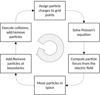
Fig. 1. The simulation cycle of a PIC/MCC bounded collisional plasma that has to be carried out several thousand times within a radiofrequency period.

As the plasmas of our interest are collisional, the PIC method (originally developed for collisionless plasmas) has to be com- plemented with the description of collision processes (as already mentioned in Section 1). For this purpose a stochastic treatment, the ‘‘Monte Carlo Collisions’’ (MCC) approach is usually adopted [3]. In this approach, colliding particles are selected in each time step randomly, based (strictly) on the probabilities of such events defined by the respective cross sections, the velocities of the particles, the background gas density and the length of the time step (see later).

The PIC/MCC method is thus a combination of two approaches.

It is capable of describing electrodynamics effects, but in most cases the electrostatic approximation provides sufficient accuracy. The method is readily applicable to 1, 2, or 3 dimensions, however, the computational load increases immensely for the higher (2 or 3) dimensions. In the following we assume a one- dimensional geometry: a source in which the plasma is estab- lished between two plane parallel electrodes, which are placed at a distanceLfrom each other. The ‘‘lateral’’ extent of the electrodes is assumed to be infinite, the plasma characteristics are therefore functions of the xcoordinate only. The velocity of the charged particles (electrons and ions are considered), is however computed in the three-dimensional velocity space upon collisions.

Because of the cylindrical symmetry of the system, however, the particles carry only the values of their axial and radial velocities, vxandvr, respectively, between their collisions with the atoms of the background gas. The superparticle weightW (that expresses how many real particles are represented by a superparticle) is the same for electrons and ions.

The electrostatic PIC/MCC scheme considered here consists of the following ‘‘elementary’’ steps (seeFig. 1), which are repeated in each time step:

• computation of the density of the particles and the total charge density at grid points,

• calculation of the potential distribution from the Poisson equation that contains the potentials of the electrodes as boundary conditions,

• interpolation of the computed electric field to the position of the particles,

• moving the particles as dictated by the equations of motion,

• identification of the particles that reach the surfaces, accounting for the interaction with the surfaces and removing them from the simulation,

• checking of the collision probabilities of the particles and executing the collision processes.

Here, we adopt an equidistant grid that has a resolution of

∆^x=L/^(M−1), whereMis the number of the grid points having coordinatesx_pwithp=0,¹,², . . .^M−1. The densities of charged particles at the points of this grid are computed with linear interpolations according to the particles’ positions as described below. The procedure applies both to electrons and ions. If the jth particle is located within thepth grid cell (p= [x_j/∆^x], where x_jis the position of thejth particle (equal either tox_e_,_jorx_i_,_jfor an electron/ion, respectively) and[·]denotes the integer part), the density increments assigned to the two grid points that surround particlejare

δⁿp=(

(p+1)∆^x−x_j) W

A∆^x², ⁽¹⁾

δⁿp+₁=(x_j−p∆^x) ^W

A∆^x², ⁽²⁾

where Ais the fictive electrode area (that is required for nor- malisation purposes only, as the ‘‘real’’ area of the electrodes is infinite). The linear interpolation scheme provides a good balance between performance and accuracy, hence why it has become the standard way to compute the particle densities at the grid points. In specific cases higher-order interpolation schemes may be used [2].

Once the particle densities at the grid points are known, the charge density at the grid points can be computed as

ρp=e(n_i_,_p−n_e_,_p), ⁽³⁾

whereeis the elementary charge,n_i_,_p andn_e_,_pare, respectively the ion and electron densities at grid point p. The potential distribution is obtained from the Poisson equation:

∇²φ= −ρ ε0

. ⁽⁴⁾

This equation can be rewritten in the following finite difference form for one-dimensional problems:

−φp−1+2φp−φp+1

∆^x² = ρp

ε0, ⁽⁵⁾

known as the Discrete Poisson Equation. Solving this equation is described in further detail in Section 4.6. Differentiating the potential distribution (Eq.(6)) we obtain the electric field at each grid point. Boundary grid points need to be treated specially as given by Eqs.(7)and(8):

E_p= φp−₁−φp+₁

2∆^x , ⁽⁶⁾

E₀= φ0−φ1

∆^x −ρ0

∆^x 2ε0

, ⁽⁷⁾

E_M−₁= φM−₂−φM−₁

∆^x +ρM−₁

∆^x 2ε0

. ⁽⁸⁾

Knowing the electric field values at the grid points allows computation of the field at the position of particlejlocated at x_j, as

E(x_j)= ^(p+1)∆^x−x_j

∆^x ^E(x^p⁾+^x^j−p∆^x

∆^x ^E(x^p⁺¹⁾. ⁽⁹⁾ The force being exerted on thejth particle located atx_jare given by

F_j=q_jE(x_j), ⁽¹⁰⁾

3

(4)

Table 1

Physical and numerical parameters of the benchmark cases.

Case

1 2 3 4

Physical parameters:

Electrode separation L[cm] 6.7 6.7 6.7 6.7

Gas pressure p[mTorr] 30 100 300 1000

Gas temperature T [K] 300 300 300 300

Voltage amplitude V [V] 450 200 150 120

Frequency f [MHz] 13.56 13.56 13.56 13.56

Numerical parameters:

Cell size ∆x L/¹²⁸ ^L/²⁵⁶ ^L/⁵¹² ^L/⁵¹²

Time step size ∆t f⁻¹/⁴⁰⁰ ^f⁻¹/⁸⁰⁰ ^f⁻¹/¹⁶⁰⁰ ^f⁻¹/³²⁰⁰

Total steps to compute NS 512 000 4 096 000 8 192 000 49 152 000

Data acquisition steps NA 12 800 25 600 51 200 102 400

Particle weight factor W 26 172 52 344 52 344 78 515

Converged computed parameters:

Number of electrons Ne 12 300 57 000 138 700 161 600

Number of ions Ni 19 300 60 200 142 300 164 500

Peak ion density nˆi[10¹⁵m⁻³] 0.140 0.828 1.81 2.57

resulting in an acceleration a_j^t = ^q^j

m_jE(x_j), ⁽¹¹⁾

which makes it possible to solve the equations of motion using, e.g., the popular leap-frog scheme, where the particle positions and accelerations are defined at integer time steps, while the velocities are defined at half integer time steps:

vjt+₁/2=vjt−₁/2+a_j^t∆^t, ⁽¹²⁾ x_j^t⁺¹=x_j^t+vjt+₁/2∆^t. ⁽¹³⁾ After updating the positions of the particles a check must be performed to identify those particles that have left the computational domain. These particles have to be removed from the ensemble.

At every time step, the probabilityP_jof thejth particle under- going a collision is given by [3]

P_j=1−exp[

n_g(x)σT(ε⁾vj∆^t]

(14) where n_g(x) is the background gas density, σT(ε) is the particle’s energy-dependent total cross-section,vjis thejth particle’s velocity and∆^tis the simulation time step. Based on the comparison ofP_jwith a random number (having a uniform distribution over the [0,1) interval) decision is made upon the occurrence of the collision. The total cross-section is given by the sum of cross-sections of all collisions the specific particle can participate in:

σT(ε⁾=

k

∑

s=₀

σs(ε⁾, ⁽¹⁵⁾

wherekis the number of reaction channels for the species of the specific particle.

There is a finite probability that a particle undergoes more than one collision within a single time step, resulting in missed collisions. For this reason the time step of the simulation must be chosen to be sufficiently small, as given by [33]:

νmax∆^t ≪1 (16)

where νmax is the maximum of the energy dependent collision frequency ν⁽ε⁾ = n_gσT(ε⁾v. Choosing a time step small enough for P_j ≈ 0.1 results in a sufficiently small number of missed collisions.

The type of the collision that occurs is chosen randomly, on the basis of the values of the cross sections of the individual possible reactions at the energy of the colliding particle. The deflection

of the particles in the collisions is also handled in a stochastic manner, see e.g. [34].

Details of the implementations of the steps described above will be discussed in parts of Section4.

The steps outlined above have to be repeated typically several thousand times per RF cycle. For sufficient accuracy the number of superparticles has to be in the order of∼ 10⁵−10⁶ in 1D simulations. The spatial grid normally consist of 100 − 1000 points. These values are dictated by the stability and accuracy requirements of the method (which are not discussed here but can be found in a number of works, e.g. [33]). Convergence to periodic steady-state condition is typically reached after thousands of RF cycles. Due to these computational requirements, in the past, such simulations were only possible on mainframe computers. Today,sequential1D simulations can be carried out on PC-class computers or workstations, with typical execution times between several hours and several weeks (depending mainly on the type and the pressure of the gas).

Ideally, the results of a PIC/MCC simulation should not depend on the number of superparticles used. In reality, however, as it was discussed by Turner [35] low particle numbers give incorrect results due to numerical diffusion in velocity space. The depen- dence of the simulation results on the number of computational particles was also analysed in [36]. The number of superparticles in our work primarily follows those used in [7], which is appropriate for a benchmarking activity, but we also executed performance measurements for higher numbers of superparticles.

It should, however, be kept in mind that for results with improved absolute accuracy the higher particle numbers should be adopted, at least in the range of few times 10⁵per species.

2.1. Benchmarks

To perform the validation of our GPU implementations we adopt the four benchmark cases that have been introduced in [7]

and compare the computed charged particle densities, being some of the most fundamental and very sensitive plasma parameters, with the reference data of [7]. The parameters of the plasma benchmark cases 1–4 are listed inTable 1.

The discharges are assumed to operate in plane-parallel geometry with one grounded and one powered electrode facing each other, therefore a spatially one-dimensional simulation can be applied. The discharge gap is filled with helium gas at densities and temperature (300 K) that are fixed for each benchmark case. A harmonic voltage waveform is applied to the powered electrode at a frequency of 13.56 MHz. The voltage amplitudes are given for each of the four benchmark cases. Charged particles

(5)

Table 2

The collision types used in our plasma model.

Reaction Type Threshold energy (eV)

e+He→e+He Elastic –

e+He→e+He* Excitation (triplet) 19.82 e+He→e+He* Excitation (singlet) 20.61 e+He→e+e+He⁺ Ionisation 24.59 He⁺+He→He⁺+He Elastic (isotropic part) – He⁺+He→He+He⁺ Elastic (backward part) –

reaching the electrodes are absorbed, and no secondary electrons are emitted. The simulated plasma species are restricted to electrons and singly charged monomer He⁺ions. Collisional processes are limited to interactions between these species and neutral helium atoms. For electron-neutral collisions, the cross section compilation known as ‘‘Biagi 7.1’’ is used [37]. This set includes elastic scattering, excitations and ionisation. Isotropic scattering in the centre of mass frame is assumed for all processes. For the ions only elastic collisions are taken into account, with an isotropic and a backward scattering channel, as proposed in [38].

The cross sections for the ions are adopted from [39]. The list of the processes is compiled inTable 2.

3. GPU programming and architecture

Modern GPUs can be programmed in a variety of ways. Ope- nACC [40] and OpenMP 4.x [15,41] provide compiler-based directives that allow a simple and iterative parallelisation of existing sequential programs, particularly if they are based on algorithms with tightly nested loops. OpenMP is platform-neutral while OpenACC has a certain bias towards NVIDIA GPUs. Devel- opers requiring tighter control of hardware resources and a more programmatic approach, can use GPU programming languages such as OpenCL [42,43] or CUDA [44,45]. These are more suited to complex algorithms and advanced performance optimisation but at the expense of increased code complexity and programming effort. OpenCL is a hardware agnostic standard supported by various vendors, utilising a portable C-based language to generate code executable on CPUs (x86/x64 and ARM architectures alike), and various accelerators including NVIDIA, AMD and Intel GPUs, and FPGAs. CUDA has a C/C++ and Fortran programming interface and can only be used on NVIDIA GPUs. To maximise programming flexibility and performance, we chose a programming language approach over directives and used both CUDA-C and OpenCL for our GPU implementations. Since the CUDA and OpenCL terminology are slightly different, in the rest of the paper we will use CUDA terminology; the matching OpenCL terms can be looked up inTable 3.

Common in both CUDA and OpenCL is the concept of the kernel, a GPU function called from the host program and exe- cuted in parallel by multiple GPU threads (a.k.a. the SIMT /Single Instruction Multiple Thread/ model). Kernel execution is an asyn- chronous operation; the CPU and GPU can execute instructions simultaneously. Synchronisation constructs are available if the GPU and CPU instructions must follow a prescribed execution order.

Every kernel call must contain two parts, (i) the list of function arguments found also in standard C functions, and (ii) the execution parameters which define the degree of parallelism.

These execution parameters are determined by an object called grid(not to be confused with a computational grid used in the PIC algorithm), which defines an index space for the individual threads to use. In theory, these grids can be N-dimensional, however, modern GPUs only support grids of up to three dimensions.

All launched threads are assigned a unique N-dimensional index

Table 3

Comparison of CUDA and OpenCL terminology.

CUDA OpenCL

GPU (device) Device

Multiprocessor Compute Unit

Scalar core Processing Element

Kernel Kernel

Global memory Global memory

Shared memory Local memory

Local memory Private memory

Grid Computation domain

Thread block Work-group

Warp Wavefront

Thread Work-item

from this grid, and executed on the GPU in groups called thread blocks.

From the architectural point of view, each GPU device consists of several Graphics Processing Clusters (GPCs) that contain a number of Streaming Multiprocessors (SMs). Each SM contains several compute cores; in modern GPUs, there are separate floating-point (FP32 and FP64), integer (INT32), special function unit (SPU) and tensor cores. These cores execute the actual instructions of a launched kernel. The number of cores is computed as the product of the number of GPCs, the number of SMs per GPC and the number of cores per SM. For instance, the number of cores in the NVIDIA V100 accelerator card is given as 6 GPCs x 10 SMs/GPC x 64 FP32/SM =5120. If we multiply the number of cores by the clock frequency of the GPU and a factor of 2 (assuming the execution of fused multiply-add /FMA/ instructions only that count as 2 operations per cycle), we obtain the approx- imate peak performance value (e.g. V100 card: 5120 cores×2 instructions/cycle×1.4 GHz≈14 TFlop/s).

Each SM has a large register file (256 kB) providing 64k registers or up to 255 registers per thread, a fast on-chip shared memory (48 or 64 kB) and an L1 cache. The shared memory is used for fast data sharing among threads running on the same SM.

Instructions are scheduled by up to four thread schedulers. Since global memory operations take in the order of 600–900 clock cycles to complete, a large number of threads is required to hide data latency. The schedulers choose threads for execution that are not stalled on data or synchronisation operations. In addition, advanced GPUs support concurrent kernel execution, as well as a number of instruction streams that help developers to maximise GPU utilisation.

3.1. Hardware environment

A wide range of GPU devices are available on the market rang- ing from gaming cards to datacentre/supercomputer accelerators.

In this paper we have used a number of GPUs representing different product classes to demonstrate their effectiveness in PIC/MCC plasma simulation and to compare their relative performance.

Table 4contains the details of the selected set of GPU cards that we used during the implementation and performance evaluation.

For each card, the table includes the number of FP32 cores, the peak computational performance, the GPU memory bandwidth values, and the HW instruction-to-byte ratio – computed aspeak performance (Gflop/s) /peak bandwidth (GB/s) – that forms the basis of the roofline performance analysis method that we use later in the paper.

The roofline performance model [46,47] provides a simple but effective tool for estimating the attainable performance and exploring the expected behaviour of parallel algorithms. If the Arithmetic Intensity (number of executed FP instructions/number of bytes read and stored) of a kernel is greater than the HW

5

(6)

Table 4

Performance characteristics of the selected GPU cards.

GPU card Cores Instruction Bandwidth HW instruction-to-

throughput (GFlop/s) (GB/s) byte ratio

NVIDIA GTX 1080 Ti 3584 11 339 484 21.91

NVIDIA GTX 1660 S 1408 5027 336 25.64

NVIDIA RTX 2080 Ti 4352 13 447 616 19.91

NVIDIA Tesla P100 3584 9340 549 14.70

NVIDIA Tesla V100 5120 14 899 900 16.55

AMD Radeon Pro WX9100 4096 12 290 483.8 25.40

AMD Radeon VII 3840 13 440 1024 13.125

Fig. 2. Roofline performance model of the selected GPU cards. Kernels with arithmetic intensity below the HW instruction-to-byte ratio are memory-bound;

the attained performance is limited by the available memory bandwidth.

instruction-to-byte ratio, the kernel is compute-bound and can potentially reach near peak performance, otherwise it is memory- bound and the performance is determined by the achieved memory bandwidth. More formally, the performance is given as AttainablePerformance[GFlop/^sec]

=min(PeakFloatingPointPerformance,

PeakMemoryBandwidth×ArithmeticIntensity), ⁽¹⁷⁾ whereArithmeticIntensity(AI) is the ratio of the executed floating point operations and the bytes transferred to/from memory in the given GPU kernel,

ArithmeticIntensity= FloatingPointOperations

Bytes_read +Bytes_written. ⁽¹⁸⁾ Some of the above parameters can be obtained from GPU specifications while others are estimated from the algorithm. When the attainable performance is plotted in function of the arithmetic intensity, a curve resembling a roof line emerges. The intersection of the two lines is at the arithmetic intensity threshold (the HW instruction-to-byte listed in Table 4) that a code must achieve to become compute-bound. Fig. 2 shows the roofline curves of the six selected GPU devices used in this paper. Note that an Arithmetic Intensity in the range of 13–26 is required to achieve maximum compute performance on these GPUs.

4. GPU implementation

In this section we discuss the details of the parallel GPU implementation of the PIC/MCC simulation core. To keep the description short and easy to follow, we will not include every detail but concentrate only on the most crucial issues. Empha- sis is placed on performance-critical design and implementation decisions.

Fig. 3. High-level structure of the parallel PIC/MCC simulation program. The host system is responsible for initialising the simulation and saving results. The actual simulation is executed exclusively on the GPU by a sequence of GPU kernel calls. Note that the final version uses restructured kernels as described in Section4.7.

4.1. Design principles

The primary goal of our work is to maximally harness the performance of the GPUs in PIC/MCC simulations. The two guiding principles in achieving this are (i) minimising execution overheads and (ii) maximising available parallelism.

As depicted in Fig. 3, our implementation uses a GPU-only simulation loop. The CPU code is used only to call the execution of the parallel GPU kernels (electron_density(), ion_density(), and so on). Since PIC simulations execute a very large number of simulation loop iterations, it is important to remove any unnecessary CPU–GPU communication inside the loop, since the PCI-e bus is a performance critical point of GPU systems. Several authors implemented hybrid systems, executing parts of the loop (e.g. the Poisson solver) on the CPU [21,48] to keep the implementation simpler. Even if the execution time of a code section might be faster on a CPU, taking all costs (CPU execution time, data transfer and synchronisation overheads) into account, the end result may not be ideal; performance suffers. We focused on implementing each step of the simulation loop on the GPU even at the cost of higher code complexity and increased programming effort.

Maximising the level of parallelism required an architecture- oriented perspective during the code design. Traditional CPU- based parallel PIC plasma simulations are based on partitioning the physical domain according to the number of cores, where each thread loops over the particles contained in a given partition.

In the 1D plasma simulation case, this coarse-grain parallelism offers speedups up to the order of 10². GPU chips, however, contain thousands of cores, generating a mismatch between the partitioning scheme and the underlying architecture. In addition, global memory operations have large latency,>⁶⁰⁰−800 clock cycles. To hide the cost of memory access, GPU programs require

(7)

Table 5

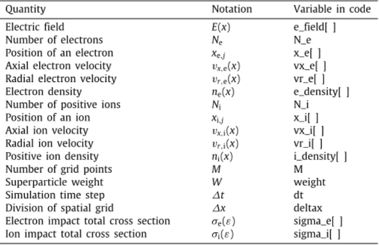
Dictionary of the notations of the physical quantities, which appear both in the theoretical part (Section2) and in the parts of the code in this section.

Quantity Notation Variable in code

Electric field E(x) e_field[ ]

Number of electrons Ne N_e

Position of an electron xe,j x_e[ ]

Axial electron velocity vx,e(x) vx_e[ ] Radial electron velocity vr,e(x) vr_e[ ]

Electron density ne(x) e_density[ ]

Number of positive ions Ni N_i

Position of an ion xi,j x_i[ ]

Axial ion velocity vx,i(x) vx_i[ ]

Radial ion velocity vr,i(x) vr_i[ ]

Positive ion density ni(x) i_density[ ]

Number of grid points M M

Superparticle weight W weight

Simulation time step ∆t dt

Division of spatial grid ∆x deltax

Electron impact total cross section σe(ε⁾ ^{sigma_e[ ]} Ion impact total cross section σi(ε⁾ ^{sigma_i[ ]}

significantly more threads than cores for efficient execution. As a rule of thumb, 10⁵−10⁶ concurrent threads are recommended for chips with few thousand cores. Consequently, instead of partitioning the physical domain, we map each particle onto an individual thread.

In the rest of this section we describe the key features of our parallel GPU implementation and discuss them from a performance optimisation perspective. The order of treatment is not the order of execution in the simulation loop; we first discuss those kernels that show performance problems but at the same time provide optimisation opportunities. Kernels that perform well or offer limited optimisations are described afterwards. To help readers connecting the implementation details to the theory and equations outlined in Section2, inTable 5we created a dictionary mapping the notation of physical quantities to the corresponding program variables.

4.2. Data structures and memory layout

The state of each type of superparticle includes its position and velocity components. In a Cartesian system, the state can be described by the tuple ⟨x, vx, vy, vz⟩. In a cylindrical coordinate system, this simplifies to⟨x, vx, vr⟩. The plasma characteristics:

the density of the charged species, the potential as well as the electric field are computed at the grid points.

There are several alternative schemes for storing particle state values. Software engineering best practices would suggest using a C structure (or a C++ class) encapsulating position, velocities and additional particle information which then can be stored in an array or list data structure (Array of Structures, AoS). Another alternative is to use special GPU data types, such as float4 havingx,y,z,welements to represent a tuple and creating arrays of these elements. The third option is to use separateN-element float arrays for individual elements of the tuple.

GPU architecture is designed in a way that memory is ac- cessed the most efficient way if consecutive threads in a thread warp access consecutive memory addresses. In other words, with this ideal, aligned and coalesced addressing pattern, a 32-thread warp can read 128 (i.e. 32 × 4) bytes either as one 128-byte or four 32-byte transactions, depending on the given GPU architecture generation. This access pattern can only be guaranteed with separate arrays for position and velocity components.

Using plain C arrays contradicts common high-level programming practices that promote encapsulation but demonstrates that high-performance parallel code often requires deviation from the software engineering methods of the sequential world. Other

Fig. 4. Data structures and their layout in GPU memory (only the electron position (x_e) and axial velocity (vx_e) arrays are shown). K blocks of 256 threads form a thread grid that are used to process all data elements. Within the blocks each number represents a thread index. Blocks are mapped to available streaming multiprocessors by the thread schedulers of the GPU. Memory access is coalesced as threads in each warp read contiguous memory addresses.

memory layouts would introduce various memory bank conflicts that drastically increase the required number of memory transactions. Since memory and computational performance is maximised if float data types are used instead of doubles, our program defaults to floats except for the density calculation and Poisson solver code sections.

Fig. 4shows the data structures used in our implementations along with illustrations how the GPU threads are mapped in units of thread blocks onto the array elements. We only show the position and velocity arrays for electrons holdingN_eelectrons.

Storing particle data in this manner results in ideal, aligned and coalesced data load/store access pattern.

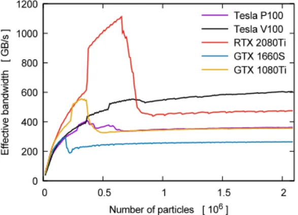
Besides access patterns, memory access efficiency is also dependent on the size of the transferred data. As shown inFig. 5, the effective memory bandwidth can be very different from the peak bandwidth values found in hardware specifications. The plots show the global memory bandwidth derived from kernel load/store operation performance in function of particle numbers.

Depending on the card chosen, a minimum of 250k to 1M particles are required for reaching maximum bandwidth. It is worth noting that most cards have a relatively narrow ’sweet spot’ range where the bandwidth is higher than the peak value. This is especially pronounced in for RTX 2080Ti card where the range is much wider (300–800k particle). We suspect this is due to memory clock boost effects and the caching mechanism. Kernels with particle counts below 100k show significantly reduced memory bandwidth, reducing the performance of memory-bound kernels even further. Fortunately, the drive for increasing the number of particles in simulations meets GPU architectural characteristics and is expected to result in increased performance.

4.3. Particle mover

In a PIC/MCC simulation, particles interact via an electric field Eformed by the superposition of an external electric field applied at the electrodes and the electric field created by the charged particles themselves. These interactions are facilitated by a computational grid in which we store information about the value of the electric field. Moreover, in every point of this grid we also store information about the electric potential φ, as well as the particle densities.

The particle mover is implemented by the GPU kernel code section below. Each GPU thread of the kernel implementing this simulation step is responsible for one particle, therefore must read one element of the input arrays x_e[tid], vx_e[tid], vr_e[tid] for electrons, and x_i[tid], vx_i[tid]|, vr_i[tid]for ions, wheretidis the thread index. In addition,

7

(8)

Fig. 5. Effective GPU global memory bandwidth (GB/s) as a function of particles to load/store.

the position x_e[tid] or x_i[tid] is used to compute the index p of the grid cell within which the particle is located.

Once the grid cell is located, the interpolated electric field value e_xis computed usinge_field[p]and e_field[p+1], from which the new velocity and position is computed by a leapfrog integration scheme. The lines computing the new velocityvxei and position xeivalues (Eqs. (12)and (13) use pre-computed constantss1=q_j∆^t/^mjanddt_e=_∆t).

// compute thread (particle) index

int tid = blockIdx.x * blockDim.x + threadIdx.x;

// load position and velocity values into register variables xei = x_e[tid]; vxei = vx_e[tid]; vrei = vr_e[tid];

// obtain grid cell index in which the particle is located int p = xei / deltax;

// calculate ...

float e_x = (((p+1)*deltax-xei) * efield[p] + (xei-p*deltax) * efield[p+1])/deltax;

// compute new velocity vxei -= s1*e_x;

// compute new position xei += vxei*dt;

check_boundary();

// store new values in global memory

x_e[tid] = xei; vx_e[tid] = vxei; vr_e[tid] = vrei;

The next step is to handle particles at the boundary of the system. When a particle leaves the system, a helper index array element (e_index[i] or i_index[i] for electrons and ions, respectively) is set to 1 to indicate to downstream stages of the calculation that this particle should be ignored in the simulation.

In our OpenCL implementation, instead of defining extra arrays, we used the fourth component of the particle velocity vector (float4datatype) to mark particles to be ignored. The kernel completes by writing out the new position and velocity values and the random number state into global memory. Our kernel is prepared for treating particles reflected back from the boundary plates, but we ignore this case for brevity.

Now, we turn our attention to the performance of this kernel.

The code ideally issues 7 load (x, vx, vr, one index element, random number state and two field values) and 4 store (x,vx,vr, random number state) requests (1 request implies 4 32-bit global memory transactions) and a number of floating-point operations (non floating-point operations are treated as overhead). Instead of hand-counting operations, profiler tools such as NVIDIAnvprof and Nsight Compute can be used to obtain the important performance metrics. In the rest of the paper, we will use the following command and a P100 card to obtain metrics.

>nvprof --metrics flop_count_sp --metrics dram_read_transactions --metrics dram_write_transactions ./executable input_parameters

From these, ArithmeticIntensity is computed as AI = flop_

count_sp/[(dram_read_transactions +dram_write_transactions)∗ 32] and gives 1.18 (electrons) and 1.16 (ions). The achieved Gflop/s rates (flop_count_sp/kernel_time) on a P100 card are 150.3 (electrons) and 98 Gflop/s (ions).Fig. 2shows that the arithmetic intensity value of 1.16 should result in approximately 500 Gflop/s performance on the P100. The low performance of this kernel is the result of the irregular memory indexing bypand p+1into the arrayefield, which causes unpredictable memory bank conflicts decreasing memory transfer performance. Nsight Compute reveals that the actual average number of memory transactions for this kernel are 35.57 (electrons) and 42.85 (ions) for loads and 12.03 (electrons) and 12 (ions) for stores. The store transactions are less than the required 16 because threads whose particles leave the system will not save output values.

Since the 1.16 arithmetic intensity is well below the optimal arithmetic intensity range of 13–26 needed for a compute-bound kernel (seeTable 4for details) we need to find ways to improve the memory data transfer performance. By utilising the on-chip shared memory, it is possible to reduce global memory bank conflicts. We modify the kernel that each thread block will read the efield array into a private shared-memory copy, then this fast shared field array will be used in the interpolation.

extern __shared__ float s_efield[];

int k = threadIdx.x;

while (k < n) {

s_efield[k] = efield[k];

k += blockDim.x;

}

__syncthreads();

// use s_efield instead of the global efield // from this point on

float e_x = ...

The benefits are that the global field array will be read in an optimal coalesced way and – while bank conflicts will remain in reading the private arrays – the much lower latency of the shared memory will improve data access performance. As a result, the number of load and store request are reduced to 5.6 and 4 and the number of transactions to 19.1 load and 12 store transactions for both electrons and ions. The arithmetic intensity remained 1.16, but the achieved performance of the kernel increased to 495.5 (electrons) and 486.6 (ions) Gflop/s, which is very close to the approx. 512 Gflop/s limit.

4.4. Collisions

The collision calculation kernel issues 8 load and 4 store requests for electrons, 7 load and 4 store requests for ions, resulting in 65 and 28 as well as 51 and 28 load/store transactions for the two types of particles. These are about twice as high as the required number of transactions at coalesced memory access. The cause of this inefficiency lies in loading theσeandσicross-section values from memory. The cross sections are stored as interpolated table values that are looked up during the computation by in- direct indexing that causes bank conflicts. In addition, since not all particles collide, thread predication due to conditional code branching also has a performance decreasing effect.

The arithmetic intensity of the electron collision kernel is 0.65, the achieved performance is 256.5 Gflop/s. The ion collision code performs better, due to its higher intensity (AI = 2.⁹²⁾ reaching 1205.6 Gflop/s performance. While both kernels show similar memory access behaviour, the higher arithmetic load in the ion collision calculation compensates memory inefficiencies to a certain degree.

(9)

4.4.1. Random number generation

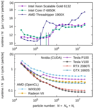
The quality and speed of random number generation in parallel Monte Carlo methods is of prime importance. In our first implementations we used vendor and community developed generators (CUDA: cuRand, OpenCL: clRNG libraries) to create uni- formly distributed random sequences for each particle. These implementations however seemed to be computationally too expensive. In the final version, we usedN =N_e+N_i independent sequences by initialising N generators based on the standard ran implementation [49] with different seeds. The statistical properties of this method were tested and found correct for our purposes. The key benefit is the approximately 3×speed gain over the library versions. For the particle number range 64k–1M, the cuRand XORWOW execution times are 35–3158µ^{s, whereas} in our implementation are 13.5–974µ^s.

4.5. Density calculations

In order to be able to calculate the potential and the electric field at the grid points the charge density corresponding to the electrons and ions has to be determined. In our scheme we distribute the density of each charged particle to two grid points between which the particle resides. The density is weighted to these two points according to the distances between the particle and the grid points. Taking one electron as example, this ‘‘charge assignment’’ procedure could be executed by the following lines of the code. The variablec_de_factorholds the pre-computed value of W/^A∆^x² stored in GPU constant memory for efficient broadcasting to all threads.

// compute thread (particle) index

int tid = blockIdx.x * blockDim.x + threadIdx.x;

// load particle position xei = x_e[tid];

// find grid cell index p = (int)(xei/deltax);

// calculate charge for grid points p and p+1 e_density[p] += (p+1)*deltax-xei)*c_de_factor;

e_density[p+1] += (xei-p*deltax)*c_de_factor;

The update instructions in the last two lines present a chal- lenging situation. Since all threads execute concurrently, appropriate locking mechanisms must be used to protect memory writes from race conditions. GPUs provide various atomic operations to handle these cases. The simplest solution is to replace the+ =operators with atomicAdd function calls. These execute the global memory read–modify–write cycle instruction sequence efficiently with built-in hardware support.

atomicAdd(&(e_density[p]), ((p+1)*deltax-xei)*c_de_factor);

atomicAdd(&(e_density[p+1]), (xei-p*deltax)*c_de_factor);

The electron and ion density kernels have reasonably high arithmetic intensities (2.69 and 3.98, respectively) but the achieved performance is rather low: 42.7 and 37.8 GFlop/s. This is the result of executing a large number of global memory atomic transactions at conflicting addresses.

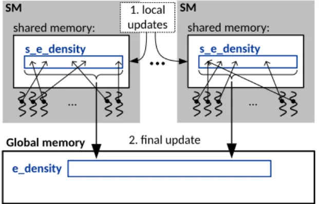
It is possible to improve this code by executing a parallel reduction operation. Each thread block (i.e. SM) will create a private density array in its on-chip shared memory as illustrated inFig. 6. Threads within the block will update values in this array by using shared-memory atomics. When all threads of the block have finished, the private arrays are written out into the global density array with global atomics.

Fig. 6.Outline of the optimised density calculation using local density arrays for each block. Once each block completed its density update using shared atomics, the shared memory arrays are written out into the main density variable in global memory with global atomic operations.

// block-local density vector

extern __shared__ float s_e_density[];

for (int i = threadIdx.x; i < n; i += blockDim.x) s_e_density[i] = 0.0f; // initialise to zero __syncthreads(); // wait for all threads to complete ...

float xei = x_e[tid];

int p = (int)(xei/deltax);

// local update in shared memory density array

atomicAdd(&(s_e_density[p]), ((p+1)*deltax-xei)*c_de_factor);

atomicAdd(&(s_e_density[p+1]), (xei-p*deltax)*c_de_factor);

__syncthreads(); // wait for all threads to complete int k = threadIdx.x;

while (k < n) { // update global memory density array atomicAdd(&(e_density[k]), s_e_density[k]);

k += blockDim.x;

}

While the code has become more complex, there are several benefits; updates are now performed in the much faster shared memory, and the number of global atomic operations is reduced from the number of particles to the number of grid cells. The final code shows increase in arithmetic intensities (3.98 and 4.22) and a significant improvement in performance (275.4 and 280 Gflop/s).

4.6. Poisson solver

Traditionally, the 1D Poisson equation is solved on CPUs using the well-known Thomas algorithm [50] that provides a solution in O(n) steps, wherenis the number of unknowns, i.e. the number of grid points. The Thomas algorithm is very efficient, requires little memory space but is inherently sequential. Consequently, in several GPU simulation implementations a hybrid execution scheme is used, i.e. the Poisson equation is solved on the CPU after the input data are copied back from the GPU memory, then once the solution is computed, the results are transferred back to the GPU memory for continuing the simulation loop.

In our implementation, we aimed to execute the solver on the GPU using a parallel algorithm to remove the data transfer overhead and make use of the parallelism the GPU offers. Two parallel solver versions were implemented and tested. The first is based on the Parallel Cyclic Reduction algorithm [51]. Our CUDA implementation is based on the GPU version introduced in [52].

The second approach that we used in our OpenCL implementation is based on the direct solution of the discrete Poisson equation.

This approach requires more memory space and requiresO(n²) steps for solution, but can be executed in parallel efficiently using matrix–vector operations.

9

(10)

Table 6

Effect of kernel performance optimisations on arithmetic intensity (AI), streaming multiprocessor (SM) and memory subsystem utilisation.

Kernel AI SM util. (%) Memory util. (%)

Original Optimised Original Optimised Original Optimised

electron_move 1.18 1.18 4.29 21.24 15.29 69.91

electron_collision 0.65 0.65 28.03 28.03 71.97 71.97

electron_density 2.69 3.98 1.01 13.45 5.25 15.87

ion_move 1.16 1.16 4.28 21.64 15.71 73.68

ion_collision 2.92 2.92 47.18 47.18 76.87 76.87

ion_density 3.98 4.22 1.22 13.69 6.28 14.30

Poisson_solver 0.05 0.05 0.41 0.41 6.1 6.1

Taking the Discrete Poisson equation (5), the solution is obtained by solving a set of linear equations which can be collec- tively written in the matrix form

Cφp= ρp∆^x²

ε0 , ⁽¹⁹⁾

where C is the coefficient matrix of the linear system andρp is the charge density atpth grid point (p = 1,², . . . ,^M−2). The solution can be written as

φp=C

−₁ρp∆^x²

ε0 . ⁽²⁰⁾

The boundary conditions at the edges of the computational domain (the first and the last grid point) are the externally imposed potentials of the electrodes. This means we only need to solveM−2 linear equations forp=1,², . . . ,^M−2.

The inverse matrixC

−₁

is constant (and symmetric) through- out the simulation, and can be precomputed as

C_sp=

{−^(s⁺^1)(M⁻^p)

M−₁ s≤p

C_ps s>^p ⁽²¹⁾

This allows us to solve Eq.(20)as a general matrix–vector multi- plication operation, which has a highly efficient implementation for GPUs.

The execution time of the Parallel Cyclic Reduction Poisson solver kernel for the grid sizes 128, 256 and 512 (benchmark cases 1–4) on the V100 system are 8.84, 9.61, 11.15 and 11.13 µs, respectively. The OpenCL direct solver kernel times (WX9100) are 18.6, 19.4, 22.9 and 22.7 µs. The sequential CPU execution times using the Thomas algorithm are 2.7 (M = 128), 3.3 (M

= 256) and 5.2 µ^{s (M} = 512) which are better than the GPU results but the overall time that includes the required additional device–host–device data transfer as well is in the range of 80–190 µ^s.

4.7. Kernel fusion

In the preceding parts we looked at the performance critical points and optimisation opportunities of the individual kernels of the PIC/MCC GPU simulation program.Table 6summarises the effects of these performance improvements in terms of arithmetic intensity, streaming multiprocessor and memory utilisation levels.

The complete simulation program has three main parts: (i) initialisation, (ii) the simulation loop, and (iii) saving states and results to file system. The initialisation stage includes data input from files and copying data to GPU memory; the simulation loop executes GPU kernels for the specified number of simulation steps; the post-processing steps include copying results from GPU to host memory then saving the results to files.

As the length of the simulation and the number of particles are changing, the relative contribution (weight) of the kernels and the host–device data transfer operations to the overall execution

Table 7

The relative contribution of individual kernels and data transfers to the overall simulation execution time. Each run is performed for 100 RF voltage cycles (V100 results).

Kernel Relative kernel execution times (%)

Case 1 Case 2 Case 3 Case 4

electron_move 7.17 7.25 7.66 8.18

electron_collision 14.25 11.89 13.17 12.81

electron_density 9.02 15.58 19.26 20.20

ion_move 7.67 7.33 8.37 8.95

ion_collision 14.15 12.35 12.13 12.40

ion_density 9.21 16.35 19.98 20.94

Poisson_solver 22.31 18.55 12.45 11.80

host-to-device copy 5.57 2.46 0.94 0.41

device-to-host copy 10.58 8.17 5.05 4.30

time changes too.Table 7lists these relative contribution values.

The purpose of this analysis is to identify kernels or memory operations that might become potential performance bottlenecks.

The particle move and density kernels increase, while the Pois- son solver and the memory copy operations decrease in weight as the number of particles and simulation steps increase (Case 1–

4). The weight of the collision kernels remain approximately the same for the different benchmarks. Overall, the particle-related kernels (electron and ion move, collision and density) represent an increasing share – from 61.5 (Case 1) to 83.5% (Case 4) – of the simulation time, indicating that further optimisations might have significant effect in reducing the simulation time.

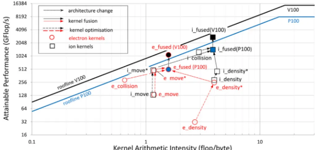
The main performance limiting factor in the particle kernels is the low arithmetic intensity. The number of arithmetic instructions cannot be increased in these kernels but if multiple kernels are fused into a single kernel, a number of load/store instructions can be reduced. For instance, the electron position is required in the e_move, e_collision and e_density kernels. In the fused kernel, we need to load the position only once, reducing memory transfer by a factor of 3. Based on this idea, we created two fused kernels, one for the electrons (electron_kernel), one for the ions (ion_kernel).Table 8lists various performance metrics of the fused kernels obtained by executing benchmark case 4. The result of kernel fusion is further time reduction. For Case 4, the execution time of the fused kernels reduced to 82.0 (electron) and 77.64 (ion)µs from the original 117.2 and 114.1 µ^{s pro-} duced by the separate electron and ion (move+collision+density) kernels. Measurements were made on a P100 card. Fig. 7 il- lustrates the effects of individual kernel optimisations and kernel fusion graphically on the roofline plot. The final, optimised fused kernels show large improvement in performance and move close to the memory-bound limit of the roofline performance curve. As a consequence, the production version of our CUDA and OpenCL PIC/MCC simulation codes are based on the fused kernel implementations.

5. Results and discussions

In this section, we first verify the correctness of our final, fused-kernel implementations by comparing them to the four