COMMENTS
ON THE EXPERIMENTAL AND THEORETICAL STUDY OF TRANSPORT PHENOMENA IN SIMPLE LIQUIDS
Stuart A. Rice* and Jean Pierre Boon*
Department of Chemistry and James Franck Institute The University of Chicago, Chicago, Illinois
and H. Ted Davis
Department of Chemistry and Department of Chemical Engineering, The University of Minnesota, Minneapolis, Minnesota
1. Introduction 252 References 253 2. Comments on the Theory of Transport Phenomena 254
2.1. Some Simple Models 255 2.2. Statistical Theories of Transport Phenomena 259
2.3. Formal Theories of Transport Phenomena 276
2.4. Phenomenological Analyses 289 2.5. Transport Properties of Liquid Mixtures 293
2.6. Comments about More Complex Liquids 314
References 317 3. Experimental Procedures and a Comparison between Theory and Observation . 320
3.1. Experimental Methods 320 3.2. Simple Liquids 324 3.3. Liquid Mixtures 337 3.4. "Complex" Liquids 352
References 359 4. Literature Survey 360
4.1. Bibliography of References 372 4.2. Supplement (1966) 399
* During 1965-66: National Science Foundation Senior Postdoctoral Fellow and Visiting Professor, Université Libre de Bruxelles, Brussels, Belgium.
+ Permanent address: Faculté des Sciences, Université Libre de Bruxelles, Brussels, Belgium.
251
1- Introduction
This review is intended to survey the available experimental data relèvent to transport phenomena in simple liquids and, wherever possible, to compare experiment with theory. For this reason, we have included an extensive survey of the literature as well as descriptions of both the experimental methods used to determine transport coefficients and the theories which may be used to calculate transport coefficients. Although it is necessary to discuss some very fundamental questions related to the nature of irreversibility in macroscopic assemblies of molecules, for the most part attention is focused on those theories that have been success- fully reduced to the point that numerical predictions of the properties of a liquid may be made. For the details of all the theories tested the reader is referred to the original literature, but sufficient information is given about the physical assumptions inherent in each analysis to render intelligible the final formulas displayed herein.
The difficulties inherent in the construction of a molecular theory of liquids are widely heralded, but probably less widely understood.
Provided that the conceptual structure of the theory is carefully defined and internally consistent, a dash of intuition can carry the theory a long way. At the present time, the theory of the equilibrium properties of a liquid* is in quantitative agreement with experiment at densities up to one-third to one-half of the normal liquid density. At higher densities the theory is qualitatively correct, but the quantitative discrepancies become large ( ~ 2 5 %, say for Ar at T = 84°K, p = 1 atm, when one compares the theoretical and experimental pressures, internal energies, etc.). For certain limiting cases, e.g., the rigid sphere fluid, theory and experiment (in this case the experiment is a computer calculation) are in essentially quantitative agreement over the entire fluid domain. Of course, the available theories of critical phenomena and phase transitions are badly inadequate, and in these cases there are qualitative differences between theory and observation.
In the preceding paragraph we hinted that a moderately satisfactory theory of liquids can be developed with the aid of intuitive constructs.
We use the words ' 'moderately satisfactory*' to indicate that a complete theory should, in principle, involve only well-defined mathematical manipulations based on transformation of the exact equations of motion, phase integral, etc. To the extent that intuitive constructs bypass mathematical difficulties, and then can later be shown to represent certain well-defined mathematical operations or approximations, a
* See, for example, Hirschfelder, Curtiss, and Bird [4] and Rice and Gray [11].
TRANSPORT PHENOMENA IN SIMPLE LIQUIDS 2 5 3
theory with intuitive content can be, more or less, transformed into a ''rigorous* ' theory. Without further apology, we shall therefore adopt the attitude that the experimental test of theoretical predictions is a valid procedure for discriminating among possible intuitive arguments, mathematical approximations, etc., even when it is, from the point of view of pure logic, inherently impossible to give a completely unambig- uous answer to the question: Which is correct ?
There have been many different attempts to construct theories of transport phenomena.* Of these, the activated state theory [2], the corresponding states theory, the statistical mechanical theory leading to kinetic equations [10, 11], the autocorrelation function theory [6, 8], and the theory of mixtures are reviewed in Section 2. Section 3 is devoted to a survey of the principles underlying the most important of the experimental methods used to determine transport coefficients, and to an examination of the experimental data. In Section 3 we attempt to define the accuracy to which the several theories describe the data, to interpret the deviations between experiment and theory, and to suggest the directions in which new experimental and theoretical work would be most valuable. The remaining section of this chapter includes a tabular display of bibliographical information and an extensive bibliography of the relevant literature.
REFERENCES
General Bibliography of Theories of Transport Phenomena:
1. S. Chapman and T. G. Cowling, "The Mathematical Theory of Non-Uniform Gases." Cambridge Univ. Press, London and New York. 1939.
2. E. S. Glasstone, K. J. Laidler, and H. Eyring, "The Theory of Rate Processes,"
Chapter 9. McGraw-Hill, New York, 1941.
3. J. Frenkel, "Kinetic Theory of Liquids." Oxford Univ. Press, London and New York, 1946.
4. J. O. Hirschfelder, C. F. Curtiss, and R. B. Bird, "The Molecular Theory of Gases and Liquids," Chapters 7-10. Wiley, New York, 1954.
5. "Transport Processes in Statistical Mechanics" (I. Prigogine, ed.) Wiley (Inter- science), New York, 1958.
6. R. Kubo, "Lectures in Theoretical Physics," Vol. 1, p. 120, Wiley (Interscience), New York, 1959.
7. S. A. Rice and H. L. Frisch, Ann. Rev. Phys. Chem. 11, 187 (1960).
8. R. W. Zwanzig, "Lectures in Theoretical Physics." Vol. 3, p. 106. (Interscience), New York, 1961.
9. N. N. Bogolubov, "Studies in Statistical Mechanics" (J. de Boer and G. E. Uhlenbeck, eds.), Vol. 1, p. 1. North-Holland Publ., Amsterdam, 1962.
* A comprehensive, but not exhaustive, bibliography is given at the end of this section.
10. I. Prigogine, *'Non-Equilibrium Statistical Mechanics." Wiley, New York, 1962;
P. Resibois, in "Many Particles Physics" (E. Meeron, ed.). Gordon and Breach, New York, 1967.
11. S. A. Rice and P. Gray, "The Statistical Mechanics of Simple Liquids." Wiley, New York, 1965.
2* Comments on the Theory of Transport Phenomena The starting point for the discussion of transport phenomena is the description of the macroscopic dissipative processes in terms of the constraints which define the nonequilibrium state of the system, and a set of coefficients which measure the rates of dissipation. Dissipative processes arise from the transport of mass, momentum, and energy. In each case there exists a phenomenological relationship between a flux and the force which is responsible for the flux. In the cases of energy and mass transport we have the Fourier and Fick equations,
(1)
with q and Jm the energy and mass fluxes, κ and D the coefficients of thermal conductivity and diffusion, T the temperature, and c the concentration of one of the two components in the medium wherein diffusion is occuring. In the case of momentum transport the stress tensor σ and the rate of strain έ play primary roles. For a Newtonian fluid the principal shearing stresses are proportional to the corresponding rates of strain and
σ = [-P + (Φ - h) V · u] 1 + 2ηί (2) with φ and η the coefficients of dilatational and shear viscosity, u the
fluid velocity, p the pressure, and 1 the unit tensor. The stress law (2) when introduced in the equation of motion of the fluid leads to the Navier-Stokes equation—the starting point for the study of fluid dynamics.
For the simple fluids considered in this book, Eqs. (1) and (2) provide an accurate representation of dissipative behavior. The coefficients Ky D, 77, and φ may be determined experimentally by a variety of methods based upon suitable solution of the appropriate differential equation (see Section 3). It is found that all of the transport coefficients vary when the temperature and density of the liquid are varied. It is observed
q dT
dt
1m
dc dt
= KVT
= KV*T
= DVc
= DV2c
TRANSPORT PHENOMENA IN SIMPLE LIQUIDS 255 that at constant external pressure D increases exponentially and η
decreases exponentially as T is increased. Under the same conditions κ is much less sensitive to changes in temperature than are η and D. For most simple liquids D is of the order of 10~5 cm2/sec, κ of the order of 10~4 cal/cm sec°C, and η of the order of 5 X 10~3 dyne sec/cm2. For liquids with extensive hydrogen bonding, such as polyhydric alcohols, η may be very much larger, as it also is for long chain molecules in general. The dilatational viscosity φ is partially responsible for the attenuation of sound in a liquid. In the case of liquid Ar, the only simple system studied to date, φ is of the same order of magnitude as η (φ/η = 1.4). For complex liquids, such as polyhydric alcohols, φ can be related to the relaxation of the internal motions of the molecules in the liquid, and can be very large in magnitude.
Suppose that, for some liquid, the several transport coefficients have been determined as a function of temperature and density. How can these data be interpreted in terms of molecular dynamics and the structure of the liquid ? The extant theories of transport phenomena, which deal with just such an analysis, may be conveniently grouped into four classes: (a) simple quasi-solid or quasi-gas models with many empirical parameters, (b) phenomenological analyses based upon the principle of corresponding states, (c) statistical mechanical theories starting from the rigorous Liouville equation but employing simplifying approximations, and (d) developments which lead to formally exact results, but which may be difficult to use for a practical calculation. In the following we examine each of these classes in detail. Mathematical details of the derivations are available in the literature and will not be repeated herein. Indeed, we shall focus attention exclusively on the nature of the physical arguments, the validity of the approximations, and the implications of the theory in other contexts. In a later section we shall also examine in detail the agreement between theory and experiment.
2.1. SOME SIMPLE MODELS
Perhaps the simplest of all descriptions of the liquid state are based on the use of quasi-crystalline model geometries. In the equilibrium theories it is usually supposed that the volume occupied by the liquid may be spanned by a virtual lattice, thereby subdividing the volume into cells. In some analyses only a single molecule can occupy a cell while in others multiple occupancy and/or zero occupancy ("holes") are included in the description. In all cases, however, the phase space available to the molecules is severely restricted by the geometric constraints expressed in terms of cell occupancy. Using the perfect lattice as the unperturbed
reference system is, superficially, an attractive suggestion. Indeed, in the case of the equilibrium theory, it may be shown that if the analysis is carried to all orders of perturbation theory, then there is obtained an exact evaluation of the canonical partition function. However, it has not proven possible to go beyond the lowest order terms in the expansion, and these provide a disappointingly poor approximation for the equilib- rium properties of liquids. Are there, then, any uses for quasi-crystalline models of the liquid state ? No completely unambiguous answer can be given to this question. In the case of equilibrium properties, quasi- crystalline models of local liquid structure may sometimes be used to advantage in the interpretation of the radial distribution function g(2)(R).
While it is recognized that long range crystalline order is absent in the liquid, the local arrangement of the neighbors of each molecule is regarded as a blurred replica of the first several coordination shells of a single crystal lattice or of a superposition of several lattice types. The number of neighbors in each diffuse coordination shell is estimated as
$ 4nR2pg{2)(R) dR under the corresponding peak of the radial distribution function, where p is the bulk density of the liquid. In this way it is inferred that, for example, the local structure of liquid mercury corresponds to an approximately close-packed array of spheres. For the case of water, the liquid is regarded as a three-dimensional net in which each water molecule is linked to four neighbours by hydrogen bonds. By superposing coordination structures of the ß-quartz, trydymite, and close-packed types, a synthetic g{2)(R) may be constructed which is in substantial agreement with experiment. At low temperatures the /?-quartz structure predominates, and at high temperatures the contribution of the close- packed structure increases.
In a similar manner the structure of liquid hydrocarbons is represented as approximating the arrangement realized in the axial close packing of slender rods. The x-ray scattering curves of aliphatic alcohols exhibit inner peaks not observed for the corresponding hydrocarbons. This peak may be qualitatively interpreted if it is assumed that the alcohol molecules are linked in chains by hydrogen bonds between the hydroxyl groups while the aliphatic groups remain approximately close packed as in the corresponding hydrocarbons.
The quasi-crystalline interpretation of the liquid pair correlation function can also be used to advantage in discussing the dielectric constant. When neighboring molecules are strongly correlated, as for example by the presence of a hydrogen bond, it can be shown that
*'(°> -
φ= W T ^ · 3 ^
2 ( 1 +*
<cos y>) (3)TRANSPORT PHENOMENA IN SIMPLE LIQUIDS 2 5 7
with n the refractive index and where <cos y> is the average of the cosine of the angle between neighboring dipoles with electric moment μ,, and there are z nearest neighbors to any dipole. Kirkwood has calculated
€'(0) = 63 for water at 300°K, whereas the observed value is 78. The predicted temperature dependence of e'(0) is also in fair agreement with observation. Similar agreement between theory and experiment is obtained when other hydrogen bonded liquids, such as the alcohols, are considered [1].
In general, quasi-crystalline models of a liquid are of most use when the correlation between molecules is very strong because of the presence of a specific orientation dependent interaction such as a hydrogen bond. For simple monatomic fluids, quasi-crystalline models are far less useful and often lead to erroneous predictions because of their inherent overestimate of the molecular ordering. For monatomic fluids, g{2)(R) computed from a quasi-crystalline model has oscillations above and below the asymptotic value of unity as much as ten molecular diameters from an arbitrary molecule, whereas the observed gi2)(R) has reached unity after only three or four molecular diameters.
In the description of transport processes the role of the quasi-lattice is more important, since the local geometry of the liquid influences the flow of mass, momentum, and energy. Consider the model used to describe diffusion. It is assumed that, in order to move, a molecule must be close to a vacant site (cell) from which it is separated by a free energy barrier. The flux of matter then depends on the rate of surmoun- ting the barrier and the concentration of vacancies. In the case of the shear viscosity, the effect of the relative motion of two planes of atoms on the frequency of atomic jumps over the barrier is used to relate the flow of momentum with the shear strain. The reader should note that in each case it is assumed that the basic step requires thermal activation, i.e., that an intermediate geometric configuration midway between the initial and final molecular structures exists, and that the ratio of the concentration of such activated states to the concentration of initial states is determined by exp(—AG*/RT) with AG% the free energy of activation. This theory predicts that D and η vary exponentially with temperature, as is observed. The quasi-crystalline theories do not relate the parameters required to calculate Dy /c, and η to the intermolecular potential or to g{2)(R) and therefore are really parametric representations rather than molecular theories. Moreover, they cannot account for the temperature dependence of D and η if the density is maintained constant rather than the pressure.
One fundamental problem raised by this representation is immediately apparent. The energy acquired by a "jumping" molecule in order that
it may pass over the free energy barrier must be dissipated in a time short relative to the passage time. If this is not true, there is a large probability that the "hot" molecule will return to its original position, and irreversibility will depend on a bias in the end points of a many- jump process. In contrast, if the "hot" molecule loses energy rapidly, then only one jump takes place and an irreversible flow is generated because any succeeding jump is uncorrelated with the jump just completed.
This picture implies the existence of a mechanism characterized by two different length scales in the free path distribution, as pointed out by Alder and Einwohner [2]: One length corresponds to the particle rattling in its cage, and the other one has the magnitude of the inter- molecular distance. Therefore the path distribution should exhibit two peaks, a conclusion which is in contradiction with the Alder and Einwohner "computer experiment" for hard spheres; i.e., the observed fluid free path distribution decays monotonically nearly as an exponential.
Furthermore, the probability of free paths of a length larger than the molecular distance is seen to be less (by many orders of magnitude) than that required by the Eyring theory to predict the diffusion coefficient.
A better picture of motion in a liquid is provided by a model proposed by Cohen and Turnbull [3]. In this model a molecule can only move if a void of critical size V* opens up adjacent to the molecule. It is supposed that such voids can occur by the occasional random coalescence of the free volume of the liquid. If σ is the diameter of a molecule, Cohen and Turnbull show that
D = {aj6)^kTjmf^ ap(-yV*IVf) (4)
where y is a numerical constant and m is the mass of the molecule. This equation qualitatively accounts for the behavior of complex molecules and provides an interpretation of the fluid behavior in the glass region where the simple form of the activated state model fails. Equation (4) does not, however, accurately describe the behavior of simple fluids. For the case of simple molecules the intermolecular repulsive potential rises much less steeply (on a scale in which the molecular diameter is the unit of length) than does the intermolecular repulsive potential of complex molecules, and this difference is one source of the errors inherent in (4).
As already hinted, of greater importance than any of the criticisms made thus far is the complete omission in the models mentioned of any attempt to understand the origin of irreversibility. Although in the theory of self-diffusion in a crystalline medium it can be shown that the jumping atom indeed does lose energy through coupling with the
TRANSPORT PHENOMENA IN SIMPLE LIQUIDS 2 5 9
surrounding lattice, no quasi-crystalline model of the liquid state includes an analysis of energy dissipation in this sense. Moreover, the complicated many-body dynamical problem which must be analyzed (in a crystal the existence of a normal mode spectrum enables this problem to be solved with satisfactory accuracy), when coupled with the formally inconsistent coupling of kinetic and statistical concepts, makes it unlikely that a logically satisfactory theory of transport in liquids can be based on the use of quasi-crystalline models. It is not a simple matter to convert the time reversible equations of motion for the molecules to a form which will yield the time irreversible fluxes (1). We shall discuss this matter in detail later. For the present we merely note that dissipative processes can be described in terms of a dynamical event, possibly complex, which is independent of prior dynamical events.
Careful consideration must be given to the nature of the molecular correlations, the relevant time scales in dissipation, and the role of perturbing forces [4].
2.2. STATISTICAL THEORIES OF TRANSPORT PHENOMENA
The development of a statistical theory of transport phenomena in liquids requires consideration of many problems, among which are:
(a) analysis of the means by which the time reversible equations of classical and quantum mechanics that are used to describe the motions of molecules lead to the time irreversible flux equations displayed in Eq. (1);
(b) derivation of a suitable kinetic equation determining the time evolution and phase dependence of some ensemble probability distribu- tion; and
(c) solution of the kinetic equation to obtain relationships between the macroscopic parameters 77, φ, κ, and D and the intermolecular potential, number density, temperature, etc.
The reader should recognize that the calculation of transport coeffi- cients is, in fact, only a small part of the general problem of describing time-dependent phenomena. Namely, it is concerned with that state of a fluid in which all time dependence resides in the local hydrodynamic flow velocity. The general problem also involves the description of those short-lived processes whose time dependence is explicit. Such processes are generally non-Markovian of a high order, and the asymptotic approach of the exact kinetic equations describing them to the Markovian equations of the hydrodynamic regime with which we are concerned in this section is discussed in Section 2.3.
As we shall see, the exact kinetic equations for a dense fluid can be displayed only in the most formal way at the present time. Consequently, their asymptotic Markovian form is unknown, and the forms of the equations derived to describe a dense fluid are based on an intuitive analysis of the nature of random processes. Indeed, at present the only kinetic equations applicable to the description of phenomena in the liquid state are those derived using the time-smoothing technique introduced by Kirkwood [5], or its equivalent.
The method of obtaining equations satisfied by the one- and two- molecule distribution functions /(1)(Γ'1 ; t)> /{2)(Γ2 ; t), respectively, is essentially that of integrating the iV-molecule distribution function /{Ν)(ΓΝ \t) over the subphase space of all the other molecules in the
system. Now, fiN) satisfies the Liouville equation, and is not known explicitly. Therefore, one may only obtain differential equations for /( 1 ) and /( 2 ) by integrating the Liouville equation term by term. The result is a coupled hierarchy of equations; i.e., the equation for/( 1 ) also involves /( 2 ), the equation for /( 2 ) also involves /( 3 ), and so on. It is necessary to truncate this hierarchy at some point in order to obtain closed equations for/«1) and/<2>.
For a classical fluid we describe the system of iV-structureless molecules in the volume V by use of the Hamiltonian equations of motion. These equations have some interesting general implications.
Since there is one equation for each degree of freedom of the system, it follows that the phase of the system at any instant is uniquely deter- mined by the phase at any other instant. In accordance with the definition of a Markovian random process, it follows that the phase of the system ΓΝ may be regarded as a Markovian process of a simple kind. (The transition probability is a δ-function, since the increment of the variable ΓΝ has only one possible value for each time instant.) The kinetic equations for the reduced distribution functions/(1),/(2),..., are concerned with the random variables ΓΊ(1), Γ2(1,2),..., which are of smaller dimensionality. Now, it is well known that the projection of a Markovian process of 6iV dimensions onto a space of smaller dimensionality (6, 12,..., dimensions) generally yields a random process of higher order.
Thus, /\(1), Γ2(1, 2),..., will be non-Markovian processes of high order.
This general feature has been obtained in the analysis of Prigogine and co-workers. They find that the stochastic interaction term has the form of a time convolution over the history of the variable. The important result is that when the system has reached a stationary state, the kinetic equations reduce to Markovian form.
At this point it is legitimate to raise the question: What is the connec- tion, if any, between the equations of hydrodynamics in microscopic or
TRANSPORT PHENOMENA IN SIMPLE LIQUIDS 261 macroscopic form and stationary states ? The first answer is obvious:
It is quite possible to discuss the hydrodynamics of a system in a nonequilibrium stationary state in which transport coefficients play a crucial role. This is a rather trivial statement, and the argument may be developed much further. The equations of hydrodynamics deal adequately with processes which are nonstationary on a macroscopic time scale. Useful results have been obtained even for such rapidly varying processes as shock waves in dilute gases. All these processes are, in fact, very slow compared to the time scale of molecular fluctuations, on which non-Markovian processes are important. Generally, one would expect that the kinetic equations should be Markovian if the processes described are sufficiently slow that local thermodynamic equilibrium is maintained in the fluid.
The problem of truncating the coupled hierarchy of kinetic equations has, therefore, two distinct features. Since an integration over the sub- phase space of (N — I) or (N — 2) molecules leaves the equations completely reversible, the truncation procedure must in the first place make the equations irreversible. Second, it must provide a means of singling out the Markovian features that the kinetic equations contain in the hydrodynamic regime. The introduction of irreversibility is not difficult; it is merely contingent upon the particular method by which the Markovian feature of the truncation is achieved. At the present time, however, no systematic procedure for obtaining the Markovian feature is known, and the one we adopt is based on that first proposed by Kirkwood [5].
Consider now the relationship between non-Markovian processes in the subphase spaces of one, two,..., molecules, and the ultimate transition to a Markovian kinetic equation defined on these same subphase spaces.
We wish to assert that an nth order process can be treated as an n-dimensional Markovian process, the reduction being accomplished by grouping the states of the process into hyperstates. Each hyperstate in the Markovian process contains information about the history of the system during the interval tm to tm+n_1. Much of this information is superfluous for the evaluation of the distribution functions in the hydrodynamic regime, but the information needed is contained within the hyperstate. The method of truncation of the hierarchy of coupled equations for the distribution functions is, therefore, a means of extracting the relevant information from the hyperstate. The particular contribution to the theory made by Kirkwood, which we have already mentioned, is the hypothesis that the relevant information for present purposes is contained in the exact distribution function averaged over an interval of time r. The average value for an interval r on the fine-grained time
scale is then associated with a single point on a coarse-grained time scale, and the process is known as coarse graining (in time*). The kinetic equations obtained in this way are, in principle, difference equations, but it turns out that the times during which changes become significant on a hydrodynamic scale are so long compared to the coarse-graining time that no significant error is introduced by treating the differences as differentials.
The introduction of irreversibility which must accompany the coarse graining is accomplished by the assumption that a time interval r exists such that the dynamical behavior of the system during one interval is related in a simple statistical manner to the dynamical events of the previous interval. It may be shown that the statistical character of the relation is sufficient to render the process irreversible.
The statistical assumption, or ansatz, can be analyzed on the basis of an intuitive picture of the dynamics of liquid molecules. Consider first the Fokker-Planck equation describing the behavior of a Brownian particle. This equation describes a stochastic process under conditions such that the transition probability (for the phase Γ of the Brownian particle) is that for a stationary Markovian process. In turn, this may be shown to be the result of allowing the time resolution of the description of the Brownian particle to be sufficiently coarse that transient behavior associated with the approach to local equilibrium in the molecular motions cannot be resolved. Thus, the description of Brownian motion as a Markovian process applies only to the discussion of processes taking place on a time scale longer than some rc characteristic of the liquid molecules. In the development of the theory rc is chosen using physical criteria such that the basic dynamical event (in this case molecular fluctuations) is statistically independent of prior events. Were this not the case, the transition probability connecting two dynamical states of the Brownian particle would not be Markovian.
The problem of Brownian motion is concerned with numerous small momentum transfers, or numerous small particle displacements. At the other extreme of behavior, where momentum transfers may frequently be large and where displacements may be large, is the dilute gas. Transport phenomena in a dilute gas are usually described by a one molecule distribution function which satisfies a kinetic equation (Boltzmann equation) in which the effects of molecular interaction appear in the form of isolated binary collisions. The rate of change of the distribution function is determined by the slow secular variations of/(1) due to streaming in phase space on which are superimposed the effects
It is possible also to coarse grain in space; similar kinetic equations are obtained.
TRANSPORT PHENOMENA IN SIMPLE LIQUIDS 2 6 3
of the binary collisions. On the average, a molecule moves a long distance (relative to its size or the range of the intermolecular forces) before undergoing an encounter. Although there is a large volume of phase space wherein there occur small angle deflections resulting from binary collisions, large angle deflections are also frequent. Indeed, large angle deflections are responsible for most of the transport of energy and momentum due to collisions.
There have been numerous attempts to derive the Boltzmann equation from the first principles of statistical mechanics with the aid of some auxiliary nonmechanical assumptions that relate to the irreversibility [5-16]. The assumptions required to effect a derivation are basically three in number: the truncation of interactions of higher order than binary collisions, the condition of molecular chaos (i.e., the condition that every pair of colliding molecules is statistically independent prior to the collision), and the slow secular variation of/(1) in space. Of these conditions, only the molecular chaos is responsible for the irreversibility.
The restriction that the singlet distribution function vary slowly in space is very mild. Even under the extreme conditions in a shock front it may be a useful approximation, and under ordinary circumstances it is certainly valid to the same extent that local parameters such as temper- ature, pressure, etc., can be employed as useful variables. The binary collision approximation is also valid in the limit of low densities, and we therefore focus attention on the question of molecular chaos and the related coarse graining.
At least part of the difficulty in analyzing the chaos property arises from the intuitive nature of this assumption. That is, the usual mental image of the gaseous collision process leads to the expectation that chaos (lack of correlation in both positions and momenta) will be produced even if absent initially, though this may require many collisions to accomplish. However, if such chaos requires a time interval corre- sponding to many collision times, then it does not lead to the Boltzmann equation which describes transport phenomena in the dilute gas. For in the Bolzmann equation the binary collisions are taken to be indepen- dent,* and the relevant time interval is therefore long compared to the duration of a collision but short compared to the mean time between collisions. The problem separates into two overlapping questions: Is the initial distribution * 'chaotic' ' and is the chaos propagated ?
Consider first the question of initial chaos. Grad has claimed that the class of functions {/™2)} which is obtained by integration of the class
* The successive collisions suffered by a particular molecule are the result of its motion through an environment which is assumed to be (statistically) unaffected by the rebounding molecules.
{/(n)} chosen to be consistent with a given singlet function/( 1 ) converges to the product/( 1 )(1)/( 1 )(2) as n -> oo [12]. The argument centers on the symmetry of the distribution function in the arguments, positions, and momenta, with the net result that the probability density is peaked in those regions of phase space for which the factorized product condition is valid. However, it is not clear that this theorem is of any use for the study of dense media, since those portions of phase space where chaos is not exhibited are just the regions most important for the description of the liquid phase. In the case of the dilute gas, where at equilibrium the pair correlation function is unity, the demonstration that the pair distribution approaches a product of singlet distributions is tantamount to the demonstration that chaos exists. Note that so far we have said nothing about the temporal or spatial scale over which chaos is to be expected. To examine this question we assume that at a given time chaos is established. It is clear that whether chaos will or will not be propagated depends in part on the time scale for which the Liouville equation is solved. Even with an initially factorized distribution, it is certainly true that for time intervals that are short compared to the mean time between collisions, a pair of molecules that has just collided will be strongly correlated with one another. It is only by the intercession of further collisions with third and fourth molecules that this correlation can be destroyed. Whereas at equilibrium, g{2) has a correlation range (i.e., a volume element within which it differs from unity) only of order of magnitude of the range of intermolecular forces, out of equilibrium the correlation range may be much larger. This is a result of the persistence of the initial state. Briefly stated, as time increases there will be an increasingly large number of initial configurations that result in collision, and thus in a certain sense the correlations grow in time. In the absence of intervening collisions the correlations for a pair of molecules are essentially constant over a distance equal to the relative velocity multi- plied by the time. Now, the derivation of the Boltzmann equation by Kirkwood [5] uses coarse graining to isolate a binary collision and define the extent of the memory of correlation. That is, the fundamental dynamical event is taken to be a binary collision and it is assumed that τ is long compared to the duration of a collision but short compared with the time between collisions. A second coarse graining is later performed upon the integrand of the collision operator. We immediately note that the formal effect of coarse graining is to limit the correlation time to r, successive intervals of length being uncorrelated. If τ is taken as long relative to the duration of an encounter, but short relative to the time between encounters, then coarse graining over an interval successfully breaks the correlations between successive collisions. This truncation is
TRANSPORT PHENOMENA IN SIMPLE LIQUIDS 2 6 5
accomplished by taking the length of the collision cylinder defining the volume of space relevant to two molecules about to collide as proportional to r. There remains, however, an indirect correlation due to the coupling through third molecules. Consider the following collision sequences:
molecule 1 collides with molecule 2, molecule 2 rebounds and collides with molecule 3, etc., the trajectories being so constructed that molecules 2 and 3 would not have collided at the time, except for the prior collision with molecule 1. It is clear that for this example molecule 1 has influenced the collision between molecules 2 and 3. For geometric reasons, the correlation due to these indirect collision sequences must decrease with increasing distance between molecules 1 and 2. That is, in a homogeneous gas, the probability that no intermediate collisions occur between the indirectly coupled collision of molecules 2 and 3 following the collision of molecules 1 and 2 is of the approximate form exp(—R12/Xf), where λ/ is the mean free path and i?12 is the distance between molecules 1 and 2, Therefore, outside a sufficiently large volume element in configuration space, the correlation due to indirect collision paths vanishes. We may now state a more restrictive condition on the time interval used for the second coarse graining. It must be chosen so as to render the correlations due to indirect collisions negligible. Note that a time interval is equivalent to a linear extension of order AR(r). Clearly, in the dilute gas, AR(T) ought to be longer than the range of the intermolecular potential but shorter than a mean free path.
The case of a dense fluid is qualitatively different. The meaning of molecular chaos in a dilute gas is that molecule 2 (which is due to collide with molecule 1) has approached molecule 1 from infinity and its distribution of possible velocities has not been affected by collisions with molecules which have recently collided with molecule 1. In a dense fluid, molecule 1 may undergo a rigid core, i.e., strongly repulsive, collision with a second molecule which has for some time past been in the region of the first coordination shell of molecule 1. Thus, molecule 2 should have an intimate statistical "knowledge" of molecule 1, and may indeed have undergone a rigid core collision with molecule 1 in the immediate past. However, if the quasi-Brownian motion produced in the molecules by the van der Waals part of the forces is sufficiently effective in causing molecule 2 to forget its previous experience, then successive rigid core collisions should satisfy the simple form of molecular chaos used.
But aside from questions of how chaos and time coarse graining are related in very short time intervals, it is pertinent to inquire how much chaos is required for the derivation of the Boltzmann equation, and whether or not chaos propagates when large time intervals are considered.
It has not yet been possible to prove in general that chaos is propagated by the Boltzmann equation although it can be shown to be true for some configurations. These configurations are just those for which the pair of molecules is widely separated and do not collide. The basic idea is that when the molecules are not close to one another,/( 2 ) a n d /( 1 )( l ) /( 2 )( 2 ) have similar time dependence. The residual difference, /( 2 ) — / (1)( 1 ) / (1)(2), can then be related to the residual differences between products of singlet distribution functions and the corresponding higher distribution functions, /( n ). When the molecules do not collide, simple rectilinear trajectories are traversed, and thereby the two molecule residuals are related to the initial values of the w-particle residuals. But if f{n) is initially chaotic, the nth. order residuals tend to zero and the time dependence of the two molecule residuals also tends to zero. Thus, the initial chaos is propagated in that set of configurations in which collisions do not occur. Due to the large correlations in the short time immediately following a collision, no general proof of the propagation of chaos has yet been constructed.
To complete this discussion of coarse graining we seek a consistency condition on the passage from the non-Markovian to the Markovian description of the fluid. In a sense, the distribution function may be thought of as a vector in a continuous space whose components represent the occupation probabilities of the various states of the phase space.
In the most general case, the probability of finding the set of states (p( n ), {n}) depends on the past history of the system. There are, however, two limiting cases where the past can be ignored [18]:
(a) If the probability for moving to the set of states denoted (p( n ), {n})(
at time t from any substate (p^, (i))t-r at time t — τ is the same for all the states of (p( n ), {n})t_T , then the probabilities for being in each substate of (p( n ), {#})/-T do not affect the outcome of the transition (P( n ), {»}).-*-(P( w ),{»})|.
(b) If, no matter what the sequence (p( n ), {n})ti, (p( n ), {n})t2 ,.··> is, we always end up with the same assignment of probabilities for being in each of the states in (p( n ), {n})(, then the preceding sequence can have no influence on the transition (p(n), {n})t_r -> (p( n ), {n})t.
These conditions are used as follows: Let it be assumed that there exists a time interval τ such that the following dynamical event, defined in r, defines a Markovian process. The dynamical event consists of a strongly repulsive binary encounter followed by a quasi-Brownian motion of the pair of molecules in the fluctuating field of all the neigh- boring molecules. Because the destruction of correlations by the quasi- Brownian motion is efficient, successive strongly repulsive encounters are
TRANSPORT PHENOMENA IN SIMPLE LIQUIDS 2 6 7
statistically independent. The compound dynamical event is, therefore, asserted to be independent of prior events of the same kind.*»+
Consider now the relationship between this hypothesis and the consistency conditions imposed by coarse graining. Which of the two limiting cases is applicable in our situation ? Consider the description of the strongly repulsive binary encounter portion of the fundamental dynamical event. The transition probability for scattering from the pair of momentum states pf, p} to px ■> p2 is a function of the impact parameter, intermolecular potential, etc. Clearly, the scattering to a set of final states px, p2 is not independent of pf, p} and, therefore, limiting case (a) is inapplicable. If coarse graining is to perform the function required we must establish that condition (b) is applicable.
If, no matter what the sequence (p( n ), {n})tl, (p( n ), {n})t2 >···> is, we always end up with the same assignment of probabilities for being in each of the states of (p( n ), {n})t, then it is necessary that the relaxation time for return to the states of (p( n ), {n})t be short relative to the time interval on which the fundamental dynamical event is defined. Thus, if it can be shown that the relaxation time for the return to local equilibrium is much shorter than the time between strongly repulsive binary encoun- ters, then the initiation of the dynamical event consisting of a strongly repulsive binary encounter followed by a quasi-Brownian motion always starts from the same distribution function. In this case the probabilities for being in each of the states of (p( n ), {n})t just define the distribution function, and the conditions of case (b) are satisfied.
A very interesting and fundamental analysis of the role of coherence time in the statistical mechanics of irreversible processes has been given by Fano [18b], using some ideas and techniques introduced by Zwanzig [18c]. Fano shows that in the limit that the dynamical coherence between a subsystem and its surroundings (reservoir) is short lived, the effective interaction between reservoir and system is weak irrespective of the magnitude of the intermolecular potential. From Fano's analysis, Hurt and Rice have developed a formal coherence time expansion for the classical fluid, and show that [19]:
(a) In the limit of short memory of dynamical coherence, the Rice- Allnatt kinetic equations (see following) are a valid description of steady state phenomena in the liquid.
* Recent studies of neutron diffraction from liquid Ar confirm the accuracy of this hypothesis (Dasamacharya and Rao [18a]).
+ The dynamical events are, of course, the interaction of the molecule, pair of molecules, etc., under consideration, with their environment. Clearly, the phase of the molecule, pair, etc., is not independent of the phase during a previous interval; it is the phase of the environment which is (assumed) independent of the phase during a previous interval.
(b) Despite the fact that the usual expansion parameters />σ3 or e/kT are not useful in the liquid, there does exist a qualitatively different expansion parameter TJT, where rc is the lifetime of dynamical corre- lations and r is the time between dynamical events. The new parameter appears naturally because, when the surrounding medium has the property of propagating away or otherwise destroying dynamical correlations in the subsystem of interest, it is not pertinent to measure the strength of the interaction in terms relating to the spacing of the continuous spectrum of the Liouville operator of the surrounding medium. All that is pertinent in this case is the lifetime of dynamical correlations. For the case of a perturbation in momentum space, Rice and Allnatt [4] have shown that the lifetime of the dynamical correlation is an order of magnitude less than the time between dynamical events, thus justifying truncation of the coherence time expansion after terms in TJT.
(c) The fundamental hypothesis of time smoothing is a natural expression of the nature of the coherence time expansion.
(d) The postulates of separability of intermolecular potential, instantaneous nature of rigid core collisions, and the nature of time smoothing all have interesting consequences for the development of Markovian kinetic equations from the exact non-Markovian statistical dynamical equations.
We have already mentioned the Rice-Allnatt kinetic equations [see (a) and (b)]. These were developed before the derivation of the coherence time expansion, using physical arguments with content substantially identical to the formal results of the coherence time analysis. For simplicity, we shall discuss the theory in intuitive terms.*
The theory of irreversible phenomena in liquids developed by Rice and Allnatt was, in the first instance, relevant to a model monatomic dense fluid in which the intermolecular potential has the form of a rigid core repulsion superimposed on an arbitrary soft potential. Subsequent analysis has shown that the extension of the model to include more realistic potentials presents no formal difficulty, provided that the repulsive potential is sufficiently short ranged.
What advantage results from separating the intermolecular potential into two parts and treating their effects separately? Quite simply, the difference in range and strength of the repulsive core and the soft potential allows the discussion of the molecular motion in terms of two
* A new derivation of these equations from a functional integral representation of nonequilibrium statistical mechanics has been given by Popielawski, Rice and Hurt [19a].
TRANSPORT PHENOMENA IN SIMPLE LIQUIDS 2 6 9
time scales: One corresponds to the large momentum and energy transfers which occur during a strongly repulsive encounter, while the other corresponds to the frequent small momentum and energy transfers which occur during the quasi-Brownian motion of a molecule in the superimposed soft force field of all the molecules in its surroundings.
The short range of the strongly repulsive core implies that the first class of encounters are of short duration, so that the probability that a molecule undergoes such encounters with two or more others simultaneously is sufficiently small that it may be neglected. The introduction of the idealized rigid core representation for this class of encounters may thus be regarded as a formal device for restricting consideration to binary encounters (i.e., rigid core encounters between not more than two molecules). It has the additional advantage of considerably simpli- fying the mathematical details of the solutions of the equations but, we believe, without significantly affecting the numerical results [20].
Irreversibility is introduced into the analysis by the use of the Kirkwood hypothesis that a time interval r exists such that the dynamical events occuring in one interval are independent of those in the preceding intervals. The dynamical event is identified as a rigid core encounter followed by erratic or quasi-Brownian motion in the fluctuating soft force field of the neighboring molecules. This identification is contingent upon the effectiveness of the quasi-Brownian motion in causing the environment to forget the momentum with which a molecule was rebounded after the rigid core encounter. This in turn implies that the relaxation time for the equilibrium of the momentum due to the soft force alone is much shorter than that due to rigid core encounters alone.
It may be shown that this physical statement is supported by detailed calculation of the appropriate relaxation times for the motion considered.
The introduction of irreversibility in the manner described leads to a set of integrodifferential equations describing the evolution of the coarse-grained singlet /( 1 )(1), doublet /( 2 )(1,2), etc., distribution functions. Details of the derivations may be found elsewhere [20].
Here, we merely quote the results:
(a) For the singlet distribution function, we find
#(!)/(!) = £ Jil) + ζ^(1)/(1)
1 = 1
where
^«/«^(-jL + l p ^ + F*·^)/.
(5)
(6)
and
F* = °<F<5>> + (1>F<*> (7) If an external force Xx acts on molecule 1, and the fluid has a hydrody-
namic velocity u, then it is easily shown that
and
^u>/(i> = Vpi . ([JjL _ u] /«» + kT Vf t/(») (8b) Of the remaining symbols in Eq. (5),
ja> = *£"(Ri ■ °) f [ / ( 1 ) ( R i p*)/<i»( R i, p*)
m J ( k - p1 2> 0 )
- /( 1 >( R i , Pi)/( 1 )(Ri. Pi)] ΡιΦ db de φ2 (9a)
(2)/
m J (k-p12>0)
+ /( 1 )(Ri , Pi) k · V j * ^ , p2)] Pl2b db de dp2 (9b) W = -L· Vi^2)(Ri ' ^ · J k[/ ( 1 )(Ri ' Pi*)/(1)(Ri > P2*)
z / w J ( k - p1 2> 0 )
+ /( 1 ,( R i . Pi)/( 1 ,(Ri, ft)] ft«* * & Φ . (9c)
with ^o2)(Ri > σ) ^ e local equilibrium pair correlation function at contact (taking the intermolecular potential to consist of a rigid core interaction plus a soft longer range interaction), k is a unit vector along the line of centers when two molecules are in contact at | R12 | = σ, σ is the rigid core diameter, b the impact parameter, and e the azimuthal angle describing the binary encounter, and the asterisk refers to values of the parameters before collision. Finally,
"<F^>=i,ÎF<f'(R1 2)^>(R1 2)rfR1 2
(10)
<»F«*> = p J* Fif'(R1 2)^»(R1, R2) «iR12
where p — (N — l)/V. It must be noted that Eq. (14) is valid only for the case that the friction coefficient ζ3 is independent of the particle
7i" = σ^) ( Κ/ 'σ ) f [/(1)(Rx. Ρί) k · V « » ^ , p*)
TRANSPORT PHENOMENA IN SIMPLE LIQUIDS 2 7 1
momentum. This is not in general true, but the full equation corre- sponding to Eq. (15) which is derived from the Rice-Allnatt theory is of such complex structure that analytic solutions are not known. In place of this general equation, Rice and Allnatt adopt, as a first approx- imation, the alternative form of the equation (which still yields the Maxwellian equilibrium momentum distribution) with constant friction coefficient. In this case the solutions to the kinetic equation may be obtained without difficulty using Kihara functions [21].
It should also be noted that the weak coupling part of the equation derived by these methods is identical with that derived by Prigogine [17].
Of course, the general theory also leads to a formal expression for the friction coefficient. Indeed, the momentum-dependent friction tensor corresponding to the weak coupling Fokker-Planck operator is found to be
.fiN-im^^rjdr^ds'ds (11) with R(A° and p{N) the position and momentum vectors for N molecules.
(b) For the doublet distribution function, if we denote the hydro- dynamic flow velocity and temperature at R^ by u^ and Ti, respectively, the final form is
#<»/<»
=£ jm
+£
WRj)^u>/(2, (12)
where the J\2) are given by (ί) J[» = /ί2,(1) + /ί2,(2)
^ ^ » ( R i . R , ) ^ )
x [ί [/<3>(R1)Pl*;R2,p2;R1)P3*;<)
LJ (k-p13>o;sym)
—/( 3 )(Ri, p! ; R2 > p2 ; Ri » Pa ; 0] ΡιΦ dh de dPs
+ f [ /( , )( R i , P i ; R , . p i ; R , . p f ; 0
J (k-p23>o;sym)
—/(3)(Ri i pi ; R2 > p2 ; R2, p3 ; 0] Ρ2Φ dh d€ dPa\ (13a)
(«) / f = n
2)d) + /<
2>(2)
= ^ ^ » ( R1 )R2) ^ ( a )
X ί ί [/"»(Rx. P x ) / " ^ > P2) k · V( 1 )( * i , p*)
L·' (k-p13>o;sym)
+ /( 1 ,( R i . Pi)/( 1 ,(R2, Λ) k · ^ i /U )( R i . P.)] As* * * Φ3
+ f [/<1>(R1, P l) / ' " ( R2 , p*) k · V2/<D(R2 , p*)
J (k-p23>o;sym)
+ /( 1 ,( R i . P i ) /a ,( R2, ft) k · V/«"(R,, p,)] PzJb db de dp3] (13b) (üi) 7i" = /?>(1) + Jj?(2)
x [ f [/«"(Rx. PÎ)/( 1 ,(R2, Ρ2) /( 1 )( ^ , P3*)
^ (k-p13>o;sym)
+/, 1 )(Ri.Pi)/, 1 ,(R2,p2)/, 1 ,(Ri,P3)]
X k · Vrf<»(Rx ; σ)/>13δ <ft rfe φ3
+ f [/( 1 ,(Ri, Pi)/(1)(R, . Pi)/( 1 )(R,. P3*)
·> (k-p23>o;sym)
+ /( 1 )( R I , P I ) /, 1 ,( R2. P 2 ) /, 1 ,( R2. P3) ]
X k · ^ « ( R , ; σ) p23b db de <fp,] (13c)
and
#<.>/(«
=[_JL + £ (J_
P i. V, + Fj» - v j ] /<« (14)
■*,(1)/(1) = Vp< · [ ( - i - P< - it,) + *T< V,J /«> (15)
F<2) = (2)p(J5T) _|_ (2)p(5) (16)
(2>p(Ä) = (2)<F(Ä)>O + (2)F(Ä)t where R = H or 5 (17) The kinetic equations (5) and (12) may be solved analytically when there are only small deviations from equilibrium. The solutions, which
TRANSPORT PHENOMENA IN SIMPLE LIQUIDS 273 depend on the temperature gradient, velocity gradient, etc., may then
be used to compute the several transport coefficients. The results are as follows.
(a) Thermal conductance:
* = «K + Kv(°) + «v(R> σ) (18) 75**Γ r 1 +(2*pofil5)g{p)
KK T Γ 1 +μπρσ>Ι5)ξ(σ) Ί (σ) Li3<2.2) + \45Csll6pmp(a)]l 32mg(a) Li2<"> + [45Csll6Pmg(a)]l
fi(2.2) = (jhrkT/myV
_ Ί5&Τ \qnpà*g{a)\ r _ J _ (2nPo*g(a)Y( 32 Y\
KÀ<T) - 32mg(a) LI 5 ) + ß<2·2» I 5 M 9**« ) \
[l+(2iyo»/5)g(a)] l Ω™
(2β<2.2> + {45isl\6mP[g(a)]}) Λ V "*" Ω™ + [45ζ3Ι\6πιΡβ(σ)]
(b) Shear viscosity:
(19)
3
τ? = % + Σ ^''(<*) +Vv(R> σ) (20)
i - l
5ΑΓ [1 + (4iw^(a)/15t>)]
^ ~ 8*(σ) [β<2·2> + (5ζ^/4^(σ)]
(2) 87rpO«g(g)*r
^ν νσ/ ~~ ΐ5 ,Q(2,2)
(21)
Γ) _ Γθ<2,2> _| ΞΜ 1 χ M _|_ 5ζ3 Γ\Αι , 4ί3«·2>
8pmfe(a)] J Λ ! ' 4ß<2-2> + ^ / ρ / η ^ σ ) ]
*<*>*) = 3&J ^.»(Ä)«*)«
with the function ^2(^) obtained as the solution to the differential equation
(W|)-W
2= ^ | (22)
dR12
with boundary conditions
12 (23)
(c) Bulk viscosity*:
4> = tû»+4>*(R>°) (24)
i=l
ΦΪ» = o
*?'(») = fv„
2)(25)
*, (Ä > σ) = ^ p* £ «'(Ä) £<*>(*) ^ Ä ) Ä» rfR (d) Ion mobility:
μ+ ~ W „ ^ (2»mm*I\™ ( 2 6 )
*·*·>£?£) +t-
where # is the charge on the ion, mi the mass of the ion, and the appro- priate value of σ is for the ion-molecule core interaction.
(e) The friction coefficient ζ3 , which appears in all the preceding formulas, has not yet been computed with comparable accuracy. Three different theoretical estimates are:
(i) is2 = ψ j V2u(R) g{2)(R) d*R (27a)
(Ü) is = - \ ( ^ - )1 / 2 n*Y2 j k*Ys(k) Ö{k) dk
* There is no kinetic contribution to the bulk viscosity; in other words: <f>k = 0.
TRANSPORT PHENOMENA IN SIMPLE LIQUIDS 275 with
Y{k) = j u(R) exp(tk · R) d3R (27b)
G(k) = | (g™(R) - 1) exp(tk · R) dm
Another estimate of the friction coefficient can be derived from the Kirkwood expression [5]
ζ = ~àrf 0 ds<F{t) ' F{t+s)> (28a)
which is the time-integrated force autocorrelation function, this function being the equilibrium ensemble average of the product of the force on a particle at time t and that on the particle at time t + s. Lebowitz and Rubin [22] and Résibois and Davis [23] have given rigorous derivations of this expression in the description of the motion of a Brownian particle.
On the other hand the use of (28a) for the description of self-diffusion of molecules of similar masses must be considered to be an approximation whose utility will be determined by comparison between experiment and theory.
Splitting the force into two parts, FiH\ a hard core interaction, and F( 5 ), a soft force, one can write the friction coefficient in the form
ί = ζπ + is + UH
+ f ds<F(t) · F<s\t + j)> + JT A<F<*>(f) · F<*>(* + i)>j. (28b) The term ζΗ is the hard core friction coefficient and in explicit form is found in the denominator of Eq. (26). Helfand [24] has evaluated ζ$ in the linear trajectory approximation, which is an evaluation of the weak coupling friction tensor given by Eq. (11). His result is that given in Eq.
(27b). Recently, Davis and Palyvos [25, 26] have evaluated ζ3 Η in the linear trajectory approximation.
The combination of the hard core result for ζΗ, Helfand's formula for
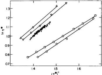
![FIG. 1. The coefficient of shear viscosity as a function of the temperature along the saturated vapor pressure curve: ( · ) Boon and Thomaes [4-15], (Δ) van Itterbeek et al](https://thumb-eu.123doks.com/thumbv2/9dokorg/1180218.86601/75.664.130.537.192.391/coefficient-viscosity-function-temperature-saturated-pressure-thomaes-itterbeek.webp)