1
Properties of Hydrogen Bonded Networks in Ethanol-water Liquid Mixtures as a Function of Temperature: Diffraction Experiments and
Computer Simulations
Szilvia Pothoczki*1, Ildikó Pethes1, László Pusztai1,2, László Temleitner1, Koji Ohara4, and Imre Bakó*3
1Wigner Research Centre for Physics, H-1121 Budapest, Konkoly Thege M. út 29-33., Hungary
2International Research Organization for Advanced Science and Technology (IROAST), Kumamoto University, 2-39-1 Kurokami, Chuo-ku, Kumamoto, 860-8555, Japan
3Research Centre for Natural Sciences, H-1117 Budapest, Magyar tudósok körútja 2., Hungary
4Diffraction and Scattering Division, JASRI, Spring-8, 1-1-1, Kouto, Sayo-cho, Sayo-gun, Hyogo 679-5198, Japan
Keywords: ethanol-water mixtures, X-ray diffraction, Molecular Dynamics simulations, H- bond statistics, Percolation
2 Abstract
New X-ray and neutron diffraction experiments have been performed on ethanol-water mixtures as a function of decreasing temperature, so that such diffraction data are now available over the entire composition range. Extensive molecular dynamics simulations show that the all- atom interatomic potentials applied are adequate for gaining insight of the hydrogen bonded network structure, as well as of its changes on cooling. Various tools have been exploited for revealing details concerning hydrogen bonding, like determining H-bond acceptor and donor sites, calculating cluster size distributions and cluster topologies, as well as computing the Laplace spectra and fractal dimensions of the networks. It is found that 5-membered hydrogen bonded cycles are dominant up to an ethanol content of 70% at room temperature, above which concentration ring structures nearly disappear. Percolation has been given special attention, so that it could be shown that at low temperature, close to the freezing point even the mixture with 90% ethanol possesses a 3D percolating network. Moreover, the water sub-network also percolates even at room temperature, with a percolation transition occurring around 50%
ethanol.
3 INTRODUCTION
Physico-chemical properties of water-ethanol solutions have been among the most extensively studied subjects in the field of molecular liquids over the past few decades1-17, due to their high biological and chemical significance. Even though they are composed of two simple molecules, the behavior of their hydrogen bonded network structures can be very complex, due the competition between hydrophobic and hydrophilic interactions.18-25 The characteristics of these networks can be greatly influenced by the concentration. Usually, three regions of the composition range are distinguished qualitatively: the water rich, the medium or transition, and the alcohol rich regions.
Most thermodynamic properties, such as excess enthalpy, isentropic compressibility and entropy, show either maxima or minima in the low alcohol concentration region, the molar ratio of ethanol xeth<0.2.26-28 Differential scanning calorimetry, NMR and IR spectroscopic studies suggested a transition point around xeth = 0.12, while additional transition points were found at xeth = 0.65 and 0.85.29-31 Concerning the intermediate region around xeth=0.5, a maximum was observed by the Kirkwood-Buff integral theory, which suggests water-water aggregation.32-35 Also, a maximum of the concentration fluctuations was found in the same region, at xeth=0.4, by small angle X-ray scattering.36
Quite recently we studied structural changes in ethanol-water mixtures as a function of temperature in the water rich region (up to xeth=0.3).23-24 There we focused mainly on the cyclic entities. We found that the number of hydrogen bonded rings has increased with lowering the temperature, and that five-fold rings were in majority, especially at xeth>0.1 ethanol concentrations.
In the present study, we extend both X-ray diffraction measurements and molecular dynamics simulations to investigating ethanol-water mixtures down to their freezing points, over the entire ethanol concentration range. Furthermore, new neutron diffraction experiments have
4
been performed in the water rich region (up to xeth=0.3). These neutron data fit nicely in the present line of investigation and support our earlier findings. The main goal here was to provide a complete picture of the behavior of the hydrogen bonded network over the entire composition range in ethanol-water mixtures, between room temperature and the freezing point. In order to identify the existence and the location of the percolation threshold, we monitor the changes of the number of molecules acting as donor or acceptor, cluster size distributions, cyclic and non- cyclic properties, and the Laplace spectra of the H-bonded network.
METHODS
X-ray and neutron diffraction experiments
Series of samples of ethanol-water mixtures have been prepared with natural isotopic abundances for synchrotron X-ray, and with fully deuterated forms of both compounds for neutron diffraction experiments.
Synchrotron experiments were performed at the BL04B237 high energy X-ray diffraction beamline of the Japan Synchrotron Radiation Research Institute (SPring-8, Hyogo, Japan).
Diffraction patterns could be obtained over a scattering variable, Q, range between 0.16 and 16 Å-1, for samples with alcohol contents of 40, 50, 60, 70, 80, 85, 90 and 100 mol % of ethanol.
Diffraction patterns have been recorded starting from room temperature and cooling down to freezing point for each composition.
Neutron diffraction measurements have been carried out at the 7C2 diffractometer of Laboratoire Léon-Brillouin38. Details of the experimental setup, the applied ancillary equipment and data correction procedure were already reported25 for methanol-water samples measured under the same conditions. For both neutron and X-ray raw experimental data, standard procedures38,39 have been applied during data treatment.
5
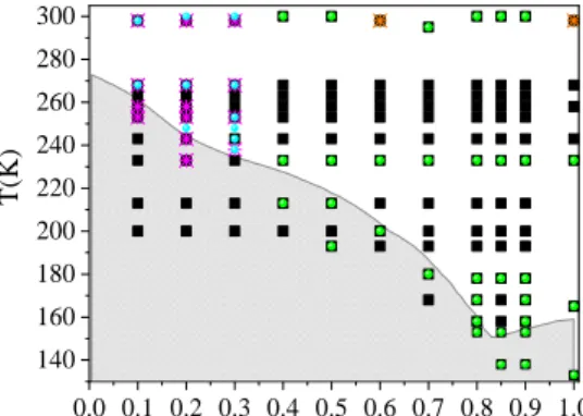
All temperature and composition points visited by the new X-ray and neutron diffraction experiments are displayed together with the phase-diagram of ethanol-water mixtures in Fig.1.
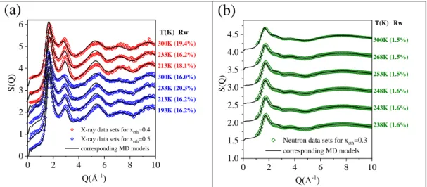
Total scattering structure factors (TSSF) obtained from the new experimental data are shown in Fig. 2 and Fig. S1.
0.0 0.1 0.2 0.3 0.4 0.5 0.6 0.7 0.8 0.9 1.0 140
160 180 200 220 240 260 280 300
T(K)
xethanol
Figure 1. Phase diagram of ethanol-water mixtures40. Gray area: solid state; white area: liquid state (as determined experimentally). Black solid squares: present MD simulations; green solid circles: new X-ray diffraction data sets; light blue solid circles: new neutron diffraction data sets; orange crosses: X-ray diffraction data sets from Ref. 19.; magenta crosses: X-ray diffraction data sets from Ref. 21.
Molecular Dynamics (MD) Simulations
Molecular Dynamics (MD) simulations were carried out by using the GROMACS software41 (version 2018.2). The Newtonian equations of motions were integrated by the leapfrog algorithm, using a time step of 2 fs. The particle-mesh Ewald algorithm was used for handling long-range electrostatic forces.42-43 The cut-off radius for non-bonded interactions was set to 1.1 nm. For ethanol molecules, the all-atom optimized potentials for liquid simulations (OPLS- AA)44 force field was used. Bond lengths were kept fixed by the LINCS algorithm45. Parameters of atom types and atomic charges can be found in Table S1. Based on results of our earlier study22, the TIP4P/200546 water model was applied, as handled by the SETTLE algorithm47.
6
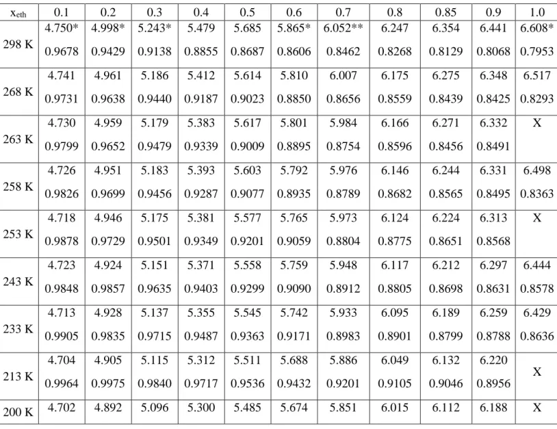
For each composition, 3000 molecules (with respect to compositions and densities) were placed in a cubic box, with periodic boundary conditions. Box lengths, together with corresponding bulk densities can be found in Table S2. All MD models studied are identified in Fig.1. Table S3 contains the various phases of the MD simulations.
RESULT AND DISCUSSION Total scattering structure factors
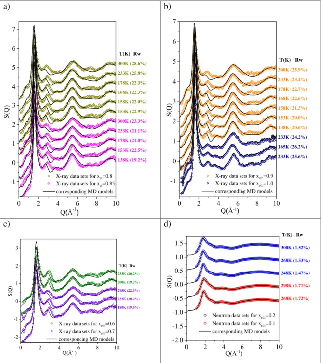
As typical examples, total scattering structure factors obtained from measured X-ray diffraction signals, for 40 mol% and 50 mol% aqueous solutions of ethanol, as a function of temperature, are drawn in Fig. 2a. Similarly, Fig. 2b shows TSSF-s from neutron diffraction for xeth=0.3.
Calculated TSSF-s are also presented in Figure 2. Additional measured TSSF-s, together with the corresponding calculated TSSF-s, can be found in Fig. S1.
0 2 4 6 8 10
0 1 2 3 4 5 6
(a)
S(Q)
Q(Å-1)
X-ray data sets for xeth=0.4 X-ray data sets for xeth=0.5 corresponding MD models
T(K) Rw 300K (19.4%) 233K (16.2%) 213K (18.1%) 300K (16.0%) 233K (20.3%) 213K (16.2%) 193K (16.2%)
0 2 4 6 8 10
1.0 1.5 2.0 2.5 3.0 3.5 4.0 4.5
(b)
Neutron data sets for xeth=0.3 corresponding MD models
T(K) Rw
300K (1.5%) 268K (1.5%) 253K (1.5%) 248K (1.6%) 243K (1.6%) 238K (1.6%)
S(Q)
Q(A-1)
Figure 2. Measured and calculated TSSF’s a) for X-ray diffraction; b) for neutron diffraction.
Agreement between calculated and measured TSSF-s for neutron diffraction appears to be almost perfect. In the case of X-ray diffraction, apparent differences can be observed, mostly around the second maximum. Rw factors were calculated to characterize differences between MD simulated [FS(Q)] (averaged over many time frames) and experimental structure factors [FE(Q)] quantitatively, thus providing a kind of goodness-of-fit (c.f. Supp. Info.). Note that
7
values of Rw for the two different experimental methods are not to be compared, due to the different data treatment procedures. It can be stated that MD models are appropriate for further analyses.
We note here that detailed analyses of partial radial distribution functions (prdf’s) are not within the scope of the present work, however all prdf’s related to H-bonding properties appear in Figs.
S2-S8.
H-bond acceptors and donors
The calculated average hydrogen bond numbers for the entire mixture and for the ethanol subsystem can be found in Figs. S9-S11. The H-bond definition applied is presented also in the Supp. Info. All of the following analyses (together with the identification of cyclic and non- cyclic entities) were performed by using our in-house computer code.48
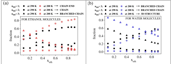
Molecules participating in H-bonds can be classified into two groups according to their roles as proton acceptors or donors. Each molecule may have a certain number of donor sites (nD) and a certain number of acceptor sites (nA), and thus can be characterized by the 'nDD:nAA ' combination. For example, ‘1D:2A’ denotes a molecule which acts as a donor of 1 H-bond and accepts 2 H-bonds. The sum of nD and nA for a given molecule provides the number of H-bonds (nHB) of that molecule. (c.f. Fig. S9.)
The most populated fractions for ethanol molecules are ‘1D:1A’, ‘1D:2A’ and the sum of
‘0D:1A’ and ‘1D:0A’ (Fig. 3a), while for water molecules they are ‘1D:2A’, ‘2D:1A’ and
‘2D:2A’ (Fig. 3b). These groups altogether contain 80% of all H-bonds at room temperature and 90% of all H-bonds at low temperatures.
8
0.2 0.4 0.6 0.8
0.0 0.2 0.4 0.6 0.8
(a) nHB= 1; at 298 K at 200 K CHAIN END nHB= 2; at 298 K at 200 K CHAIN
nHB= 3; at 298 K at 200 K BRANCHED CHAIN
fraction
xeth
FOR ETHANOL MOLECULES
0.2 0.4 0.6 0.8
0.0 0.2 0.4 0.6 0.8
(b) nHB= 3; at 298 K at 200 K BRANCHED CHAIN nHB= 3; at 298 K at 200 K BRANCHED CHAIN nHB= 4; at 298 K at 200 K 3D STRUCTURE
fraction
xeth
FOR WATER MOLECULES
Figure 3. Donor and acceptor sites a) for ethanol molecules and b) for water molecules as a function of ethanol concentration.
Concerning ethanol molecules, the occurrence of the ‘1D:1A’ combination is above 50% over almost the entire concentration range, independently of the temperature. This group corresponds to chain-like arrangements, which become more preferred with increasing ethanol content and at lower temperatures. It is remarkable that in the water-rich region the ‘1D:2A’
combination has the same as (xeth=0.2), or even a slightly higher occurrence (xeth=0.1) than that of ‘1D:1A’. With decreasing water content, the occurrence of ‘1D:2A’ decreases. Also, this group is more dominant at 200 K.
Water molecules most often behave according to the ‘2D:2A’ scheme. The occurrence of this arrangement significantly increases with decreasing temperature, as well as with increasing water content. On the other hand, the fractions of ‘1D:2A’ and ‘2D:1A’ combinations increase as temperature increases. There is a well-defined asymmetry between these two (‘1D:2A’ and
‘2D:1A’) types of water molecules in terms of their populations, which difference becomes more pronounced with increasing ethanol concentration. The fractions of ‘1A:1D’ for ethanol molecules, ‘1D:2A’ for ethanol molecules, ‘2D:1A’ for water molecules, ‘2D:2A’ for water molecules as a function of temperature can be found in Fig. S12. Furthermore, calculated H- bond number excess parameter is shown in Fig. S13.
9 Clustering and percolation
Two molecules are regarded as members of a cluster, according to the definitions introduced by Geiger et al.49, if they are connected by a chain of hydrogen bonds. Concerning the pure components of the mixtures studied here, water molecules are forming a three dimensional percolating hydrogen bonding network46,49, whereas in pure ethanol only chain (or branched chain) structures can be detected.50,51
There are several descriptors connected to the properties of networks that can be used for the determination of the percolation transition. This work focuses on the cluster size distribution (P(nc)). However, very similar conclusions may be drawn from scrutinizing several other parameters such as the average largest cluster size (C1), average second largest cluster size (C2), and the fractal dimension of the largest cluster (fd). More detailed discussion is provided in the Supporting Information, below Fig. S14.
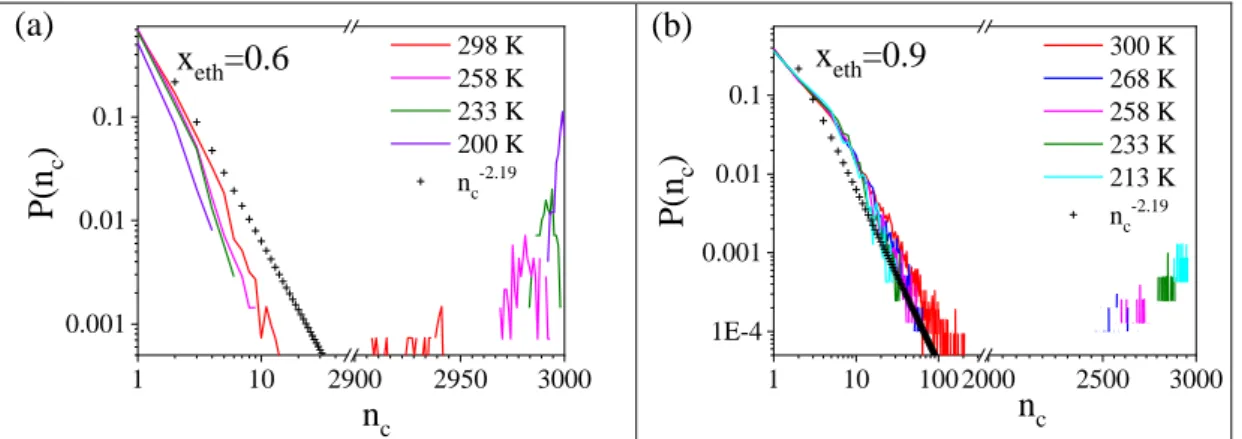
Cluster size distributions are shown in Figure 4. The system is percolated when the number of molecules in the largest cluster is in the order of the system size. For random percolation on a 3D cubic lattice, the cluster size distribution can be given by P(nc)=nc-2.19 (nc is the number of molecules in a given cluster).52,53 Percolation transition can be ascertained by comparing the calculated cluster size distribution function of the present system with that obtained for the random one. At each temperature up to xeth=0.85 (Fig. 4 and Fig. S15a) a well-defined contribution can be found at large cluster size values, signaling percolation. Systems with xeth=0.9 (Fig. 4b) show the same behavior at lower temperatures, but this signature disappears at room temperature. This suggests that in the latter case the system is close to the percolation threshold, which can be expected between 0.9 and 1.0 ethanol molar fraction. Ethanol molecules in the pure liquid compose non-percolated assemblies (Fig. S15b).2,8,20
10
1 10 2900 2950 3000
0.001 0.01 0.1
(a) 298 K
258 K 233 K 200 K nc-2.19
P(nc)
nc xeth=0.6
1 10 100 2000 2500 3000
1E-4 0.001 0.01 0.1
(b) 300 K
268 K 258 K 233 K 213 K nc-2.19
P(n c)
nc xeth=0.9
Figure 4. Cluster size distributions from the room temperature to the lowest studied temperature a) for xeth=0.6, b) for xeth=0.9.
The role of water molecules was then analyzed separately. All of the four quantities mentioned above for characterizing the percolation transition were calculated, taking into account only H- bonds between water molecules. Fig. 5 shows one representation. The average largest cluster size divided by the total number of water molecules drops down below 0.5, which the sign of the percolation transition, between xeth=0.4 and xeth=0.5 at 300 K, and between xeth=0.5 and xeth=0.6 at 200 K, respectively. Similar values were found for percolation in formamide-water54 and glycerol-water mixtures55. However, in those cases both of the constituents (not only water molecules) form 3D percolating H-bonded networks in the liquid state. Here, in contrast, independently of the concentration, ethanol molecules form only short chain-like structures, but not large percolated networks. Typical hydrogen bond network topologies for the largest cluster at the composition of xeth=0.4, 0.7 and 0.9 are shown in Fig. S16.
0.2 0.4 0.6 0.8
0.0 0.2 0.4 0.6 0.8 1.0
largest cluster/total
xeth
11
Figure 5. The average largest cluster size divided by the total number of water molecules, as a function of the ethanol concentration. Black open square symbols: 300 K, red solid square symbols: 200 K.
Rings and chains
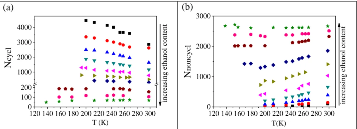
Hydrogen bonded clusters may contain non-cyclic, chain-like and cyclic, “closed into themselves” entities (c.f. Fig. S16). The number of cyclic entities (Ncycl), the number of molecules (Nnoncycl) that are not members of any ring (nc< 10) and the cyclic size distribution (nr) were calculated using the algorithms developed by Chihaia et al.56
Figure 6 summarizes the numbers of cyclic and non-cyclic entities as a function of ethanol concentration and temperature. The number of cycles decreases significantly with increasing ethanol content. As a result, in the ethanol rich region (above 70 mol%) mostly non-cyclic entities are present. Both the Nnoncycl and Ncycl entities show a strong temperature dependence up to around xeth=0.80-0.85. This effect appears to be more pronounced for non-cyclic entities.
At the highest ethanol concentrations, where most of the molecules are arranged in chains, the number of chains formed is independent of temperature.
120 140 160 180 200 220 240 260 280 300 0
100 200 1000 2000 3000 4000
(a)
increasing ethanol content
Ncycl
T (K)
120 140 160 180 200 220 240 260 280 300 0
1000 2000 3000
(b)
increasing ethanol content
Nnoncycl
T(K)
Figure 6. a) Number of cyclic entities, and b) number of non-cyclic entities as a function of ethanol concentration and temperature. Black squares: xeth=0.1; red circles: xeth=0.2; blue up triangles: xeth=0.3; dark cyan down triangles: xeth=0.4; magenta left triangles: xeth=0.5; dark
12
yellow right triangles: xeth=0.6; navy diamonds: xeth=0.7; dark red pentagons: xeth=0.8; dark magenta hexagons: xeth=0.85; green stars: xeth=0.9.
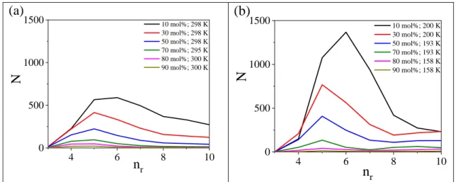
It has already been demonstrated that in pure water, molecules prefer to form six-membered rings at room temperature, which behaviour becomes more pronounced during cooling.24 This statement remains true in ethanol-water mixtures (Fig. 7), as well, as long as the ethanol molar ratio stays around 0.1, whereas for xeth=0.2 and 0.3, 5-membered rings become dominant22. Regardless of the ethanol concentration, there are always more rings at low temperatures22,24. Focusing now on mixtures with ethanol contents higher than 30 mol%, 5-membered rings take the leading role up to a concentration somewhere between xeth=0.7 and 0.8, where the number of rings (per particle configuration) falls below 100. These tendencies are more pronounced at lower temperatures.
Note that for the sake of comparison, results for the region between xeth=0.1 and 0.3 are also presented in Figure 7, although detailed discussions of ring size distributions for the water rich region can be found in Ref. 22. The new element here is that the corresponding curves are consistent also with our fresh neutron diffraction data (cf. Fig. 2b).
4 6 8 10
0 500 1000
(a)1500
10 mol%; 298 K 30 mol%; 298 K 50 mol%; 298 K 70 mol%; 295 K 80 mol%; 300 K 90 mol%; 300 K
N
nr 4 6 8 10
0 500 1000
(b)1500
10 mol%; 200 K 30 mol%; 200 K 50 mol%; 193 K 70 mol%; 193 K 80 mol%; 158 K 90 mol%; 158 K
N
nr
Figure 7. Ring size distributions as a function of xeth. a) At room T; b) at the studied lowest T.
13 Spectral properties of H-bonded networks
It has already been shown that Laplace spectra57-67 of H-bonded networks is a good topological indicator for monitoring the percolation transition in liquids68. Several authors have studied the relationship between the eigenvector corresponding to the second smallest eigenvalue (λ2) and the graph structure; well documented reviews can be found in the literature.58,62,65 More details are placed in Supp. Info.
Figure 8 provides Laplace spectra of ethanol-water mixtures as a function of concentration at room temperature. The low λ values (up to 0.3) are enlarged at the bottom. Spectra of the pure constituents can be found in Ref. 68. According to the topology of the H-bonded network, two cases can be distinguished in connection with Laplace-spectra: (1) For liquids whose molecules are forming a 3D percolated network, a well-defined gap can be detected at low eigenvalues.
(2) For systems without extended 3D network structure, where molecules link to each other so that to construct (branched) chains, several well-defined peaks (λ= 0.5,1, 1.5, 2…etc.) show up, without any recognizable gap at low eigenvalues. Pure water falls into the first category, while pure liquid ethanol belongs to the second one.68
Concerning the mixtures studied here, the existence of the gap mentioned above depends on composition. Up to an ethanol content of 95 % a well-defined gap can be found. However, above 95% ethanol content this gap disappears. Concerning the H-bond network, this means that there is a limiting alcohol concentration beyond which the presence of chains of molecules is dominant. In this concentration region, percolated networks cannot be detected. That given concentration when percolation vanishes can be considered as a percolation threshold. At concentrations lower than this limiting value, water-like 3D percolated networks are formed.
At lower temperatures no percolation threshold could be found, all systems have 3D network structures (cf. Fig. 4b).
14
0.0 0.1 0.2 0.3
0.1 1 10
0 2 4 6 8
0.1 1 10
P(
l)
l
Figure 8. The Laplace spectra of ethanol-water mixtures as a function of concentration at room temperature. Black line: xeth=0.1; red line: xeth=0.4; blue line: xeth=0.95.
SUMMARY AND CONCLUSIONS
X-ray and neutron diffraction measurements have been conducted on ethanol-water mixtures, as a function of temperature, down to the freezing points of the liquids. As a result of the new experiments, temperature dependent X-ray structure factors are now available for the entire composition range.
For interpreting experimental data, series of molecular dynamics simulations have been performed for ethanol-water mixtures with ethanol contents between 10 mol% and 90 mol%.
Temperature has been varied between room temperature and the freezing point of the actual mixture. With the aim of evaluating the applied force fields, MD models have been compared to new X-ray diffraction data over the entire composition range, as well as to new neutron diffraction experiments over the water rich region. It has been established that the combination of OPLS-AA (ethanol) and TIP4P/2005 (water) potentials have reproduced individual experimental data sets, as well as their temperature dependence, with a more than satisfactory accuracy. It may therefore be justified that the MD models are used for characterizing hydrogen bonded networks that form in ethanol-water mixtures.
15
When H-bond acceptor and donor roles of water molecules are taken into account, the occurrence of the ‘2D:2A’ combination increases linearly at every concentration with decreasing temperature.
The percolation threshold and its variation with temperature has been estimated via various approaches: we found that even at the highest alcohol concentration, the entire system percolates at low temperatures. The percolation transition for the water subsystems was found to be a 3D percolation transition that occurs between xeth=0.4 and xeth=0.5 at 300 K, and between xeth=0.5 and xeth=0.6 at 200 K, respectively.
Concerning the topology of H-bonded assemblies, in mixtures with ethanol contents higher than 30 mol%, 5-membered ring take the leading role up to the xeth=0.7 and 0.8, where the number of rings falls dramatically. This tendency is most pronounced at low temperatures.
Supporting Information
Measured and calculated total scattering structure factors for X-ray diffraction for the ethanol- water mixtures as a function of temperature (Fig. S1); Lennard-Jones parameters and partial charges for the atom types of ethanol used in the MD simulations (Table S1); Steps of Molecular Dynamics simulation at each studied temperature (Table S2); Box lengths (nm), corresponding bulk densities (g/cm3) for each simulated system (Table S3); Selected partial radial distribution functions for the mixture with 40 mol%, 50 mol%, 60 mol%, 70 mol%, 80 mol%, 85 mol% and 90 mol% ethanol as a function of temperature (Figs. S2-S8); Average H-bond numbers considering each molecule, regardless of their types, together with the case when considering water–water H-bonds only (Fig. S9); Average H-bond number for ethanol-ethanol subsystem (Fig. S10); Average H-bond numbers considering connections of water molecules only, as well as considering connections of ethanol molecules only (Fig. S11); Fraction of donor and acceptor
16
sites as a function of temperature (Fig. S12); H-bond number excess parameter (Fig. S13); The average largest cluster size (C1) and average second largest cluster size (C2) as a function of ethanol concentration and temperatures in ethanol-water mixtures (Fig. S14); Cluster size distributions from the room temperature to the lowest studied temperature a) for xeth=0.85, b) for pure ethanol (Fig. S15); Typical hydrogen bonded network topologies in water-ethanol mixtures at concentrations xeth = 0.40 (left), 0.70 (middle), and 0.90 (right) (Fig. S16); Values of the inequality calculated by Equation 4. Black open squares: left side of Eq. 4 at 298 K; black solid squares: right side of Eq. 4 at 298 K; red open circles: left side of Eq. 4 at 233 K; red solid circles: right side of Eq. 4. at 233 K (Fig. S17).
AUTHOR INFORMATION Corresponding Authors
Szilvia Pothoczki – Wigner Research Centre for Physics, H-1121 Budapest, Konkoly-Thege M. út 29-33., Hungary; Email: pothoczki.szilvia@wigner.hu
Imre Bakó – Research Centre for Natural Sciences, H-1117 Budapest, Magyar tudósok körútja 2., Hungary; Email: bako.imre@ttk.hu
Authors
Ildikó Pethes – Wigner Research Centre for Physics, H-1121 Budapest, Konkoly-Thege M.
út 29-33., Hungary;
László Pusztai – Wigner Research Centre for Physics, H-1121 Budapest, Konkoly-Thege M.
út 29-33., Hungary; International Research Organization for Advanced Science and
Technology (IROAST), Kumamoto University, 2-39-1 Kurokami, Chuo-ku, Kumamoto, 860- 8555, Japan
17
László Temleitner – Wigner Research Centre for Physics, H-1121 Budapest, Konkoly -hege M. út 29-33., Hungary;
Koji Ohara – Diffraction and Scattering Division, JASRI, Spring-8, 1-1-1, Kouto, Sayo-cho, Sayo-gun, Hyogo 679-5198, Japan
Acknowledgement
The authors are grateful to the National Research, Development and Innovation Office (NRDIO (NKFIH), Hungary) for financial support via grants Nos. KH 130425, 124885 and FK 128656.
Synchrotron radiation experiments were performed at the BL04B2 beamline of SPring-8 with the approval of the Japan Synchrotron Radiation Research Institute (JASRI) (Proposal Nos.
2017B1246 and 2018A1132). Neutron diffraction measurements were carried out on the 7C2 diffractometer at the Laboratoire Léon Brillouin (LLB), under Proposal id. 378/2017. Sz.
Pothoczki and L. Temleitner acknowledge that this project was supported by the János Bolyai Research Scholarship of the Hungarian Academy of Sciences. The authors thank J. Darpentigny (LLB, France) for the kind support during neutron diffraction experiment. Valuable assistance from Ms. A. Szuja (Centre for Energy Research, Hungary) is gratefully acknowledged for the careful preparation of mixtures.
18 References
(1) Ghoufi, A.; Artzner, F.; Malfreyt, P. Physical Properties and Hydrogen-Bonding Network of Water−Ethanol Mixtures from Molecular Dynamics Simulations. J. Phys. Chem. B 2016, 120, 793−802.
(2) Mijaković, M.; Polok, K. D.; Kežić, B.; Sokolić, F.; Perera, A; Zoranić, L. A comparison of force fields for ethanol–water mixtures. Molecular Simulation 2014, 41, 1-14.
(3) Miroshnichenko, S.; Vrabec, J. Excess properties of non-ideal binary mixtures containing water, methanol and ethanol by molecular simulation. J. Mol. Liq. 2015, 212, 90-95.
(4) Dixit, S.; Crain, J.; Poon, W.; Finney, J.; Soper, A. K. Molecular Segregation Observed in a Concentrated Alcohol-Water Solution. Nature 2002, 416, 829-832.
(5) Noskov, S.; Lamoureux, G.; Roux, B. Molecular Dynamics Study of Hydration in Ethanol-Water Mixtures Using a Polarizable Force Field. J. Phys. Chem. B 2005, 109, 6705- 6713.
(6) Požar, M.; Bolle, J.; Sternemann, C.; Perera, A. On the X-ray Scattering Pre-peak of Linear Mono-ols and the Related Microstructure from Computer Simulations. J. Phys. Chem.
B 2020, 124, 38, 8358–8371.
(7) Požar, M.; Lovrinčević, B.; Zoranić, L.; Primorać, T.; Sokolić, F.; Perera, A. Micro- heterogeneity versus clustering in binary mixtures of ethanol with water or alkanes. Phys.
Chem. Chem. Phys. 2016, 18, 23971−23979.
(8) Požar, M.; Perera, A. Evolution of the micro-structure of aqueous alcohol mixtures with cooling: A computer simulation study. J. Mol. Liq. 2017, 248, 602-609.
(9) Halder, R.; Jana, B. Unravelling the Composition-Dependent Anomalies of Pair
Hydrophobicity in Water−Ethanol Binary Mixtures. J. Phys. Chem. B 2018, 122, 6801–6809.
19
(10) Lam, R. K.; Smith, J. W.; Saykally, R. J. Communication: Hydrogen bonding interactions in water-alcohol mixtures from X-ray absorption spectroscopy. J. Chem. Phys. 2016, 144, 191103.
(11) Stetina, T. F.; Clark, A. E.; Li, X. X-ray absorption signatures of hydrogen-bond structure in water–alcohol solutions. Int. J. Quantum. Chem. 2019, 119, e25802.
(12) Soper, A. K.; Dougan, L.; Crain, J.; Finney, J. L. Excess Entropy in Alcohol−Water Solutions: A Simple Clustering Explanation. J. Phys. Chem. B 2005, 110, 3472-3476.
(13) Wakisaka, A.; Matsuura, K. Microheterogeneity of ethanol-water binary mixtures observed at the cluster level. J. Mol. Liq. 2006, 129, 25−32.
(14) Nishi, N.; Koga, K.; Ohshima, C.; Yamamoto, K.; Nagashima, U.; Nagami, K.:Molecular association in ethanol-water mixtures studied by mass spectrometric analysis of clusters generated through adiabatic expansion of liquid jets. Journal of the American Chemical Society 1988, 110, 5246-5255.
(15) Frank, H. S.; Evans, M. W.; Free Volume and Entropy in Condensed Systems III. Entropy in Binary Liquid Mixtures; Partial Molal Entropy in Dilute Solutions; Structure and Thermodynamics in Aqueous Electrolytes. J. Chem. Phys. 1945, 13, 507−532.
(16) Böhmer, R.; Gainaru, C.; Richert, R. Structure and dynamics of monohydroxy alcohols—
Milestones towards their microscopic understanding, 100 years after Debye. Physics Reports 2014, 545, 125–195.
(17) Koga, Y.; Nishikawa, K.; Westh, P. Icebergs” or No “Icebergs” in Aqueous Alcohols?:
Composition-Dependent Mixing Schemes. J. Phys. Chem. A 2004,108, 3873-3877.
(18) Choi, S.; Parameswaran, S; Choi, J-H. Understanding alcohol aggregates and the water hydrogen bond network towards miscibility in alcohol solutions: graph theoretical analysis.
Phys. Chem. Chem. Phys 2020, 22, 17181-17195.
20
(19) Gereben, O.; Pusztai, L. Investigation of the Structure of Ethanol-Water Mixtures by Molecular Dynamics Simulation I: Analyses Concerning the Hydrogen-Bonded Pairs. J. Phys.
Chem. B 2015, 119, 3070-3084.
(20) Gereben, O.; Pusztai, L. Cluster Formation and Percolation in Ethanol-Water mixtures.
Chem. Phys. 2017, 496, 1-8.
(21) Takamuku, T.; Saisho, K.; Nozawa, S.; Yamaguchi, T. X-ray diffraction studies on methanol–water, ethanol–water, and 2-propanol–water mixtures at low temperatures. J. Mol.
Liq. 2005, 119, 133-146.
(22) Pothoczki, Sz.; Pusztai, L.; Bako, I. Variations of the Hydrogen Bonding and of the Hydrogen Bonded Network in Ethanol-Water Mixtures on Cooling. J. Phys. Chem. B 2018, 122 (26), 6790–6800.
(23) Pothoczki, Sz.; Pusztai, L.; Bako, I. Temperature dependent dynamics in water-ethanol liquid mixtures. J. Mol. Liq. 2018, 271, 571-579.
(24) Bakó, I.; Pusztai, L.; Temleitner, L. Decreasing temperature enhances the formation of sixfold hydrogen bonded rings in water-rich water-methanol mixtures. Scientific Reports 2017, 7, 1073.
(25) Pethes, I.; Pusztai, L.; Ohara, K.; Kohara, S.; Darpentigny, J.; Temleitner, L.
Temperature-dependent structure of methanol-water mixtures on cooling: X-ray and neutron diffraction and molecular dynamics simulations. J. Mol. Liq. 2020, 314, 113664.
(26) Sato, T., A. Chiba, and R. Nozaki. Dynamical aspects of mixing schemes in ethanol—
water mixtures in terms of the excess partial molar activation free energy, enthalpy, and entropy of the dielectric relaxation process. J. Chem. Phys. 1999, 110, 2508-2521.
(27) Ott, J. B.; Stouffer, C. E.; Cornett, G. V.; Woodfield, B. F.; Wirthlin, R. C.; Christensen, J. J.; Deiters, U. K. Excess enthalpies for (ethanol + water) at 298.15 K and pressures of 0.4, 5, 10, and 15 MPa. The Journal of Chemical Thermodynamics, 1986, 18, 1-12.
21
(28) Wormald, C. J.; Lloyd, M. J. Excess enthalpies for (water + ethanol) at T= 398 K to T=
548 K and p= 15 MPa. The Journal of Chemical Thermodynamics, 1996, 28, 615-626.
(29) Pradhan, T.; Ghoshal, P.; Biswas, R. Structural transition in alcohol-water binary mixtures: A spectroscopic study. J. Chem. Sci. 2008, 120, 275−287.
(30) Nishi, N.; Takahashi, S.; Matsumoto, M.; Tanaka, A.; Muraya, K.; Takamuku, T.;
Yamaguchi, T.: Hydrogen-Bonded Cluster Formation and Hydrophobic Solute Association in Aqueous Solutions of Ethanol. The Journal of Physical Chemistry 1995, 99, 462-468.
(31) D'Angelo, M.; Onori, G.; Santucci, A. Self-association of monohydric alcohols in water:
compressibility and infrared absorption measurements, J. Chem. Phys. 1994, 100, 3107.
(32) E. Matteoli; L. Lepori. Solute–solute interactions in water. II. An analysis through the Kirkwood–Buff integrals for 14 organic solutes. J. Chem. Phys. 1984, 80, 2856.
(33) Perera, A.; Sokolić, F.; Almásy, L.; Koga, Y. Kirkwood-Buff integrals of aqueous alcohol binary mixtures. J. Chem. Phys. 2006, 124, 124515.
(34) Marcus, Y. Preferential Solvation in Mixed Solvents. Part 5. Binary Mixtures of Water and Organic Solvents. J. Chem. Soc., Faraday Trans. 1990, 86, 2215–2224.
(35) Ben-Naim, A. Inversion of the Kirkwood–Buff theory of solutions: application to the water–ethanol system. J. Chem. Phys. 1977, 67, 4884.
(36) Nishikawa, K. and Iijima, T. Small-angle x-ray scattering study of fluctuations in ethanol and water mixtures. The Journal of Physical Chemistry 1993, 97, 10824-10828.
(37) Kohara, S.; Suzuya, K.; Kashihara, Y.; Matsumoto, N.; Umesaki, N.; Sakai, I. A horizontal two-axis diffractometer for high-energy X-ray diffraction using synchrotron
radiation on bending magnet beamline BL04B2 at SPring-8. Nucl. Instruments Methods Phys.
Res. Sect. A 2001, 467–468, 1030-1033.
(38) Cuello, G. J.; Darpentigny, J.; Hennet, L.; Cormier, L.; Dupont, J.; Homatter, B. et al. 7C2, the new neutron diffractometer for liquids and disordered materials at LLB. J. Phys. Conf. Ser. 2016, 746 012020.
22
(39) Kohara, S.; Itou, M.; Suzuya, K.; Inamura, Y.; Sakurai, Y.; Ohishi, Y.; Takata, M.
Structural studies of disordered materials using high-energy x-ray diffraction from ambient to extreme conditions. J. Phys. Condens. Matter 2007, 19, 506101.
(40) Flick, E. W., Ed. Industrial solvents handbook, Fifth Edition; Noyes Data Corporation, Westwood, New Yersey, USA. 1998.
(41) van der Spoel, D.; Lindahl, E.; Hess, B.; Groenhof, G.; Mark, A. E.; Berendsen, H. J.
GROMACS: fast, flexible, and free, J. Comp. Chem. 2005, 26, 1701.
(42) Darden, T.; York, D.; Pedersen, L. Particle mesh Ewald: An N⋅log(N) method for Ewald sums in large systems. J. Chem. Phys. 1993, 98, 10089.
(43) Essman, U.; Perera, L.; Berkowitz, M. L.; Darden, T.; Lee, H.; Pedersen, L. G. A smooth particle mesh Ewald method. J. Chem. Phys. 1995, 103, 8577.
(44) Jorgensen, W. L.; Maxwell, D.; Tirado-Rives, S. Development and Testing of the OPLS All-Atom Force Field on Conformational Energetics and Properties of Organic Liquids J. Am.
Chem. Soc. 1996, 118, 11225-11236.
(45) Hess, B.; Bekker, H.; Berendsen, H. J. C.; Fraaije J.G.E.M. LINCS: A linear constraint solver for molecular simulations. J. Comp. Chem. 1997, 18, 1463-1472.
(46) Abascal, J. L. F.; Vega, C. A. A general purpose model for the condensed phases of water:
TIP4P/2005. J. Chem. Phys. 2005, 123, 234505.
(47) Miyamoto, S.; Kollman, P. A. Settle: An analytical version of the SHAKE and RATTLE algorithm for rigid water models. J. Comput. Chem. 1992, 13, 952-962.
(48) Bakó, I.; Megyes, T.; Bálint, Sz.; Grósz, T.; Chihaia, V. Water–methanol mixtures:
topology of hydrogen bonded network. Phys. Chem. Chem. Phys. 2008, 10, 5004-5011.
(49) Geiger, A.; Stillinger, F. H.; Rahman, A. Aspects of the percolation process for hydrogen‐bond networks in water. J. Chem. Phys. 1979, 70,4185.
23
(50) Cardona, J.; Sweatman, M. B.; Lue, L. Molecular Dynamics Investigation of the
Influence of the Hydrogen Bond Networks in Ethanol/Water Mixtures on Dielectric Spectra.
J. Phys. Chem. B 2018, 122, 1505−1515.
(51) Guevara-Carrion, G.; Vrabec, J.; Hasse, H. Prediction of self-diffusion coefficient and shear viscosity of water and its binary mixtures with methanol and ethanol by molecular simulation J. Chem. Phys. 2011, 134, 074508.
(52) Malthe-Sorenssen, A. Percolation and Disordered Systems – A Numerical Approach, Springer, 2015.
(53) Jan, N. Large lattice random site percolation, Physica A 1999, 266, 72.
(54) Bakó, I.; Oláh, J.; Lábas, A.; Bálint, S.; Pusztai, L.; Bellissent-Funel, M.-C. Water- formamide mixtures: Topology of the hydrogen-bonded network. J. Mol. Liq. 2017, 228, 25- 31.
(55) Towey, J. J.; Soper A. K.; Dougan L. What happens to the structure of water in cryoprotectant solutions? Faraday Discuss. 2013, 167, 159-176.
(56) Chihaia, V.; Adams, S.; Kuhs, W. F. Molecular dynamics simulations of properties of a (0 0 1) methane clathrate hydrate surface. Chem. Phys. 2005, 317, 208-225.
(57) Van Mieghem, P. Graph Spectra for Complex Networks. Cambridge University Press, 2010.
(58) Cvetkovic, D.; Simic, S. Graph spectra in Computer Science. Linear Algebra Appl. 2011, 434, 1545–1562.
(59) Von Luxburg, U. A tutorial on spectral clustering. Stat. Comput. 2007, 17, 395-416.
(60) Chung, F. Spectral Graph Theory. Chapter 2.2. A.M.S. CBMS, Providence, Rhode Island, 1997.
(61) Banerjee, A.; Jost, J. On the spectrum of the normalized graph Laplacian. Linear Algebra Appl. 2008, 428, 3015-3022.
24
(62) McGraw, P. N.; Menzinger, M. Laplacian spectra as a diagnostic tool for network structure and dynamics. Phys. Rev. E 2008, 77, 031102.
(63) Hata, S.; Nakao, H. Localization of Laplacian eigenvectors on random networks. Sci.
Rep. 2017, 7, 1121.
(64) Julaiti, A.; Wu, B.; Zhang, Z. Eigenvalues of normalized Laplacian matrices of fractal trees and dendrimers: analytical results and applications. J. Chem. Phys. 2013, 138, 204116.
(65) de Abreu, N. M. M. Old and new results on algebraic connectivity of graphs. Linear Algebra Appl. 2007, 423, 53–73.
(66) Fiedler, M. A property of eigenvectors of nonnegative symmetric matrices and its applications to graph theory. Czech. Math. J. 1975, 25, 619-633.
(67) Friedman, J. Some geometric aspects of graphs and their eigenfunctions. Duke Math J.
1993, 69, 487-525.
(68) Bakó, I.; Pethes, I.; Pothoczki, Sz.; Pusztai, L. Temperature dependent network stability in simple alcohols and pure water: The evolution of Laplace spectra. J. Mol. Liq. 2019, 273, 670–675.
25
Supporting Information for
Properties of hydrogen bonded network in ethanol-water liquid mixtures as a function of temperature: diffraction experiments and computer simulations
Szilvia Pothoczki*1, Ildikó Pethes1, László Pusztai1,2, László Temleitner1, Koji Ohara4, and Imre Bakó*3
1Wigner Research Centre for Physics, H-1121 Budapest, Konkoly Thege M. út 29-33., Hungary
2International Research Organization for Advanced Science and Technology (IROAST), Kumamoto University, 2-39-1 Kurokami, Chuo-ku, Kumamoto, 860-8555, Japan
3Research Centre for Natural Sciences, H-1117 Budapest, Magyar tudósok körútja 2., Hungary
4Diffraction and Scattering Division, JASRI, Spring-8, 1-1-1, Kouto, Sayo-cho, Sayo-gun, Hyogo 679-5198, Japan
*E-mail: pothoczki.szilvia@wigner.hu; Phone: +36 1 392 2222/ext. 1469
*E-mail: bako.imre@ttk.hu; Phone: +36 1 382 6981
26
Figure S1: Measured and calculated total scattering structure factors (TSSF’s) for the ethanol-water mixtures as a function of temperature. a) X-ray diffraction TSSF’s for xeth=0.8 and 0.85; b) X-ray diffraction TSSF’s for xeth=0.9 and 1.0; c) X-ray diffraction TSSF’s for xeth=0.6 and 0.7; d) neutron diffraction TSSF’s for xeth=0.1 and 0.2.
a)
0 2 4 6 8 10
-1 0 1 2 3 4 5 6 7
X-ray data sets for xet=0.8 X-ray data sets for xet=0.85 corresponding MD models
T(K) Rw 300K (28.6%) 233K (25.8%) 178K (22.3%) 168K (22.3%) 158K (22.0%) 153K (22.9%) 300K (23.3%) 233K (21.1%) 178K (21.0%) 153K (22.5%) 138K (19.2%)
S(Q)
Q(Å-1)
b)
0 2 4 6 8 10
-1 0 1 2 3 4 5 6 7
T(K) Rw
300K (25.9%) 233K (23.4%) 178K (22.7%) 168K (22.6%) 158K (21.3%) 153K (20.0%) 138K (20.6%) 233K (24.2%) 165K (26.2%) 233K (25.6%)
S(Q)
Q(Å-1)
X-ray data sets for xeth=0.9 X-ray data sets for xeth=1.0 corresponding MD models
c)
0 2 4 6 8 10
-2 -1 0 1 2 3
S(Q)
Q(Å-1)
X-ray data sets for xeth=0.6 X-ray data sets for xeth=0.7 corresponding MD models
T(K) Rw
233K (20.2%) 200K (19.2%) 295K (22.3%) 233K (20.2%) 180K (19.0%)
d)
0 2 4 6 8 10
-2.0 -1.5 -1.0 -0.5 0.0 0.5 1.0 1.5
Neutron data sets for xeth=0.2 Neutron data sets for xeth=0.1 corresponding MD models
T(K) Rw
300K (1.52%) 268K (1.53%) 248K (1.47%) 298K (1.71%) 268K (1.72%)
S(Q)
Q(A-1)
27
Table S1: Lennard-Jones parameters and partial charges for the atom types of ethanol used in the MD simulations.
Atom types σ (Å) ε (kJ/mol) q (e)
C (H3) 3.5 0.276144 -0.18
C (H2) 3.5 0.276144 0.145
H 2.5 0.12552 0.06
O 3.12 0.71128 -0.683
OH 0 0 0.418
Table S2: The first rows: box lengths (nm), the second rows: the corresponding bulk densities (g/cm3) for each simulated system. One star symbol: at 298; two stars symbol: at 295 K; without symbol: at 300 K.
xeth 0.1 0.2 0.3 0.4 0.5 0.6 0.7 0.8 0.85 0.9 1.0
298 K
4.750*
0.9678
4.998*
0.9429
5.243*
0.9138
5.479 0.8855
5.685 0.8687
5.865*
0.8606
6.052**
0.8462
6.247 0.8268
6.354 0.8129
6.441 0.8068
6.608*
0.7953 268 K
4.741 0.9731
4.961 0.9638
5.186 0.9440
5.412 0.9187
5.614 0.9023
5.810 0.8850
6.007 0.8656
6.175 0.8559
6.275 0.8439
6.348 0.8425
6.517 0.8293 263 K
4.730 0.9799
4.959 0.9652
5.179 0.9479
5.383 0.9339
5.617 0.9009
5.801 0.8895
5.984 0.8754
6.166 0.8596
6.271 0.8456
6.332 0.8491
X
258 K
4.726 0.9826
4.951 0.9699
5.183 0.9456
5.393 0.9287
5.603 0.9077
5.792 0.8935
5.976 0.8789
6.146 0.8682
6.244 0.8565
6.331 0.8495
6.498 0.8363 253 K
4.718 0.9878
4.946 0.9729
5.175 0.9501
5.381 0.9349
5.577 0.9201
5.765 0.9059
5.973 0.8804
6.124 0.8775
6.224 0.8651
6.313 0.8568
X
243 K
4.723 0.9848
4.924 0.9857
5.151 0.9635
5.371 0.9403
5.558 0.9299
5.759 0.9090
5.948 0.8912
6.117 0.8805
6.212 0.8698
6.297 0.8631
6.444 0.8578 233 K
4.713 0.9905
4.928 0.9835
5.137 0.9715
5.355 0.9487
5.545 0.9363
5.742 0.9171
5.933 0.8983
6.095 0.8901
6.189 0.8799
6.259 0.8788
6.429 0.8636 213 K
4.704 0.9964
4.905 0.9975
5.115 0.9840
5.312 0.9717
5.511 0.9536
5.688 0.9432
5.886 0.9201
6.049 0.9105
6.132 0.9046
6.220 0.8956
X 200 K 4.702 4.892 5.096 5.300 5.485 5.674 5.851 6.015 6.112 6.188 X
28
0.9976 1.0053 0.9948 0.9782 0.9672 0.9502 0.9365 0.9260 0.9132 0.9096
193 K X X X X
5.473 0.9739
5.670 0.9524
5.841 0.9415
6.010 0.9285
6.092 0.9223
6.172 0.9169
X
180 K X X X X X X
5.826 0.9488
X X X X
178 K X X X X X X X
5.974 0.9455
6.073 0.9309
6.151 0.9261
X
168 K X X X X X X
5.819 0.9519
5.972 0.9463
6.067 0.9338
6.147 0.9278
X
165 K X X X X X X X X X X
6.295 0.9199
158 K X X X X X X X
5.970 0.9471
6.051 0.9413
6.121 0.9400
X
153 K X X X X X X X X
6.043 0.9451
6.098 0.9505
X
138 K X X X X X X X X
6.029 0.9517
6.082 0.9581
X
133 K X X X X X X X X X X
6.259 0.9358
29
Table S3: Steps of Molecular Dynamics simulation at each studied temperature. (After energy minimization the initial box was heated up to 340 K in order to avoid the aggregation of ethanol molecules. The stages of the simulation series for each composition were the following at each studied temperature (even at 340 K).)
Type Run time (ns)
Thermostat time const.
T (ps)
Barostat time const.
p (ps)
NPT_short 2 BerendsenS1 0.1 Berendsen 0.1
NPT_long 10 Nose-HooverS2-S3 1.0 Parrinello-RahmanS4 4.0
NVT_short 1 Berendsen 0.1
NVT_long 5 Berendsen 0.5
All results were derived from NVT_long simulations. In each case the TSSF-s were calculated also from the simulated models, using simulated partial radial distribution functions, by an in- house code. For calculating partial radial distribution functions the g_rdf software was used, that is part of the GROMACS software package.
Goodness-of-fit:
𝑅𝑊[𝐹(𝑄)] = √∑ (𝐹𝑆(𝑄𝑖)−𝐹𝐸(𝑄𝑖))𝑖
∑ 𝐹𝐸𝑖 (𝑄𝑖) ), where FS(Q) is the calculated value from the MD simulation, FE(Q) is the experimental structure factor.
(S1) Berendsen, H. J. C.; Postma, J. P. M.; DiNola, A.; Haak, J. R. Molecular dynamics with coupling to an external bath. J. Chem. Phys. 1984, 81, 3684.
(S2) Nose, S. A molecular dynamics method for simulations in the canonical ensemble. Mol. Phys. 1984, 52, 255- 268.
(S3) Hoover, W. G. Canonical dynamics: Equilibrium phase-space distributions. Phys. Rev. A 1985, 31, 1695.
(S4) Parrinello, M.; Rahman, A. Polymorphic transitions in single crystals: A new molecular dynamics method. J.
Appl. Phys. 1981, 52, 7182.
30
Figure S2: Selected partial radial distribution functions for the mixture with 40 mol % ethanol as a function of temperature.
2 4 6 8 10 12
0.0 0.5 1.0 1.5
298 K 258 K 233 K 200 K
g O
eth-O
w(r)
2 4 6 8 10 12
0.0 0.5 1.0 1.5
x eth =0.40
4 6 8 10 12
0.0 0.5 1.0
g O
w-(O)H
eth(r) g O
w-O
w(r)
g O
eth-H
w(r) g O
eth-(O)H
eth(r)
2 4 6 8 10 12
0.0 0.5 1.0 1.5 2.0
4 6 8 10 12
0 1 2
r(Å) 2 4 6 8 10 12
0 1 2 3
g O
w-H
w(r)
r(Å)
31
Figure S3: Selected partial radial distribution functions for the mixture with 50 mol % ethanol as a function of temperature.
2 4 6 8 10 12
0.0 0.5 1.0 1.5
298 K 258 K 233 K 200 K
g O
eth-O
w(r)
2 4 6 8 10 12
0.0 0.5 1.0 1.5
x eth =0.50
4 6 8 10 12
0.0 0.5 1.0
g O
w-(O)H
eth(r) g O
w-O
w(r)
g O
eth-H
w(r) g O
eth-(O)H
eth(r)
2 4 6 8 10 12
0.0 0.5 1.0 1.5 2.0
4 6 8 10 12
0 1 2
r(Å)
2 4 6 8 10 12
0 1 2 3
g O
w-H
w(r)
r(Å)
32
Figure S4: Selected partial radial distribution functions for the mixture with 60 mol % ethanol as a function of temperature.
2 4 6 8 10 12
0.0 0.5 1.0 1.5
298 K 258 K 233 K 200 K
g O
eth-O
w(r)
2 4 6 8 10 12
0.0 0.5 1.0 1.5
x eth =0.60
4 6 8 10 12
0.0 0.5 1.0
g O
w-(O)H
eth(r) g O
w-O
w(r)
g O
eth-H
w(r) g O
eth-(O)H
eth(r)
2 4 6 8 10 12
0.0 0.5 1.0 1.5 2.0
4 6 8 10 12
0 1 2
r(Å) 2 4 6 8 10 12
0 1 2 3
g O
w-H
w(r)
r(Å)
33
Figure S5: Selected partial radial distribution functions for the mixture with 70 mol % ethanol as a function of temperature.
2 4 6 8 10 12
0.0 0.5 1.0 1.5
298 K 258 K 233 K 200 K
g O
eth-O
w(r)
2 4 6 8 10 12
0.0 0.5 1.0 1.5
x eth =0.70
4 6 8 10 12
0.0 0.5 1.0 1.5
g O
w-(O)H
eth(r) g O
w-O
w(r)
g O
eth-H
w(r) g O
eth-(O)H
eth(r)
2 4 6 8 10 12
0.0 0.5 1.0 1.5 2.0 2.5
4 6 8 10 12
0 1 2 3
2 4 6 8 10 12
0 1 2 3
r(Å)
g O
w-H
w(r)
r(Å)
34
Figure S6: Selected partial radial distribution functions for the mixture with 80 mol % ethanol as a function of temperature.
2 4 6 8 10 12
0.0 0.5 1.0
1.5 298 K
258 K 233 K 200 K 158 K
g O
eth-O
w(r)
2 4 6 8 10 12
0.0 0.5 1.0 1.5
x eth =0.80
4 6 8 10 12
0.0 0.5 1.0
g O
w-(O)H
eth(r) g O
w-O
w(r)
g O
eth-H
w(r) g O
eth-(O)H
eth(r)
2 4 6 8 10 12
0 1 2 3
4 6 8 10 12
0 1 2 3
r(Å) 2 4 6 8 10 12
0 1 2 3
g O
w-H
w(r)
r(Å)
35
Figure S7: Selected partial radial distribution functions for the mixture with 85 mol % ethanol as a function of temperature.
2 4 6 8 10 12
0.0 0.5 1.0
1.5 298 K
258 K 233 K 200 K 158 K
g O
eth-O
w(r)
2 4 6 8 10 12
0.0 0.5 1.0 1.5
x eth =0.85
4 6 8 10 12
0.0 0.5 1.0 1.5
g O
w-(O)H
eth(r) g O
w-O
w(r)
g O
eth-H
w(r) g O
eth-(O)H
eth(r)
2 4 6 8 10 12
0 1 2 3
4 6 8 10 12
0 1 2 3
r(Å) 2 4 6 8 10 12
0 1 2 3
g O
w-H
w(r)
r(Å)
36
Figure S8: Selected partial radial distribution functions for the mixture with 90 mol % ethanol as a function of temperature.
2 4 6 8 10 12
0.0 0.5 1.0
1.5 298 K
258 K 233 K 200 K 158 K
g O
eth-O
w(r)
2 4 6 8 10 12
0.0 0.5 1.0 1.5
x eth =0.9
4 6 8 10 12
0.0 0.5 1.0 1.5
g O
w-(O)H
eth(r) g O
w-O
w(r)
g O
eth-H
w(r) g O
eth-(O)H
eth(r)
2 4 6 8 10 12
0 1 2 3
4 6 8 10 12
0 1 2 3
r(Å) 2 4 6 8 10 12
0 1 2 3
g O
w-H
w(r)
r(Å)
37 H-bond definition
Two molecules were considered hydrogen bonded (1) if they were found at a distance r(O···H)
< 2.5 Å and H-O…O angle < 30° or (2) if they were found at a distance r(O···H) < 2.5 Å and the interaction energy between molecules was more negative than -3 kcal/mol (ca. -12 kJ/mol).
In the latter case H-bond interactions are taken into account as attractive interactions. Note that results only with the “energetic” definition are presented in this work: the two definitions were in good agreement and the energetic definition, whenever it is available, is thought to be more robust.
The average number of hydrogen bonds (nHB) in the mixtures (Figure S9), when taking into account all the connections, decreases when the ethanol content increases. At each concentration nHB linearly increases with decreasing temperature. Water subsystems follow this tendency, but only at ethanol concentrations lower than 60 mol%. At higher concentrations the number of H-bonds between water pairs is almost constant. This latter statement is, independently from the ethanol concentration, also true for the ethanol subsystem (Fig. S10) over the entire temperature range investigated.
Figure S9. Average H-bond numbers considering each molecule, regardless of their types, together with the case when considering water–water H-bonds only.
140 160 180 200 220 240 260 280 300 0.5
1.0 1.5 2.0 2.5 3.0 3.5
10 mol% 50 mol% 80 mol%
20 mol% 60 mol% 85 mol%
30 mol% 70 mol% 90 mol%
40 mol% circle: nHB(wat-wat); star: nHB (all-all)
n HB
T(K)
38
Figure S10: Average H-bond number for ethanol-ethanol subsystem.
140 160 180 200 220 240 260 280 300 0.5
1.0 1.5
10 mol% 50 mol% 80 mol%
20 mol% 60 mol% 85 mol%
30 mol% 70 mol% 90 mol%
40 mol%
n HB
T(K)
The number of H-bonded neighbors around (central) water and (central) ethanol molecules (Fig.
S11) varies linearly with temperature at all concentrations. The only exception is the two highest ethanol concentrations (85 mol% and 90 mol%) below 190 K, where nHB becomes constant.
Figure S11 Average H-bond numbers considering connections of water molecules only, as well as considering connections of ethanol molecules only.
140 160 180 200 220 240 260 280 300 1.5
2.0 2.5 3.0 3.5 4.0
H-bonds of ethanol molecules
10 mol% 40 mol% 70 mol% 90 mol%
20 mol% 50 mol% 80 mol%
30 mol% 60 mol% 85 mol%
n HB
T (K)
H-bonds of water molecules