PCCP PAPER

PCCP PAPER

Received 00th January 20xx, Accepted 00th January 20xx DOI: 10.1039/x0xx00000x www.rsc.org/

A general formulation of the quasiclassical trajectory method for reduced-dimensionality reaction dynamics calculations

Tibor Nagy^a*, Anna Vikár^a, György Lendvay^a,b*

Dimension reduction by freezing the unimportant coordinates is widely used in intramolecular and reaction dynamics calculations when the solution of the accurate full-dimensional nuclear Schrödinger equation is not feasible. In this paper we report on a novel form of the exact classical internal-coordinate Hamiltonian for full and reduced-dimensional vibrational motion of polyatomic molecules with the purpose of using it in quasiclassical trajectory (QCT) calculations. The derivation i s based on the internal to body-fixed frame transformation, as in the t-vector formalism, however it does not require the introduction of rotational variables to allow cancellation of non-physical rotations within the body-fixed frame. The formulas needed for QCT calculations: normal mode analysis and state sampling as well as for following the dynamics and normal- mode quantum number assignment at instantaneous states are presented. The procedure is demonstrated on the CH4, CD4, CH3D and CHD3 isotopologs of methane using three reduced-dimensional models, which were previously used in quantum reactive scattering studies of the CH4+XCH3+HX type reactions. The reduced-dimensional QCT methodology formulated this way combined with full-dimensional QCT calculations makes possible the classical validation of reduced-dimensional models that are used in the quantum mechanical description of the nuclear dynamics in reactive systems [Vikár et al., J.

Phys. Chem. A 120 (2016) 5083–5093.].

1. Introduction

Dimension reduction is often used in modeling phenomena in chemical physics to reduce the complexity of the model. By selecting the degrees of freedom that are relevant to the investigated properties of the system, one can concentrate the effort on a model whose smaller size allows one to perform a simulation at a higher level of sophistication. In molecular physics, reduced-dimensional (RD) models have been used in the description of nuclear motion both in rovibrational spectroscopy^1,2 as well as in molecular^3–5 and reaction dynamics simulations^6–17. In both cases, the possibility of simplification is offered by the separation of time scales and the weakness of the coupling between the various modes of nuclear motion.

In vibrational spectroscopy, the semi-rigid modes are well described by the normal mode approximation^18–20 in which the potential and kinetic energies are considered as quadratic functions of Cartesian or internal coordinates and of the conjugate momenta, resp.. The description of large amplitude motion (LAM), in floppy molecules, such as hindered rotor type modes, however, require a more sophisticated treatment,

because the quadratic approximation does not work, often within the space swept by the zero-point motion. The frequencies of such modes are generally much smaller than those of stiffer vibrations, and the potential coupling between the fast and slow degrees of freedom is often also limited. A way to achieve a numerically feasible description of vibration of molecules with LAMs is that one reduces the dimensionality of the problem to those of the strongly anharmonic low-frequency modes by freezing the fast vibrations^1,2.

In molecular dynamics simulation of, for example, biomolecules in water, when a large number of solvent molecules are present, the high-frequency OH stretching vibrations require the integration time step to be small.

However, their instantaneous phase has no effect on the much slower conformational motion, thus one can freeze them,^4,5 which allows a significantly faster, yet realistic simulation of the system.

In reaction dynamics, the reactive event often concerns a small number of internal coordinates involving only a few atoms, called active modes, and the rest are considered as

“spectators”. Dimension reduction is possible because the potential- and often the kinematic coupling between the active and spectator modes are small. In the corresponding scattering calculation the active degrees of freedom are treated explicitly, while the coordinates of spectator modes are frozen at their values at the saddle point of the potential energy surface (PES) or at the equilibrium geometry of reactant molecules. In quantum and state-to-state quasiclassical dynamical calculations it is necessary to know the quantum states of the reactants and products, for which one needs to properly

a.Institute of Materials and Environmental Chemistry, Research Centre for Natural Sciences, Hungarian Academy of Sciences, Magyar tudósok körútja 2., H-1117 Budapest, Hungary. E-mail: nagy.tibor@ttk.mta.hu,lendvay.gyorgy@ttk.mta.hu

b.Department of General and Inorganic Chemistry, University of Pannonia, Egyetem u. 10, H-8800 Veszprém, Hungary.

†Electronic Supplementary Information (ESI) available: Method of Lagrange multipliers for holonomic and scleronomic constraints. An efficient form of constraints allowing simple analytic gradients and Hessians. See DOI: 10.1039/x0xx00000x

ARTICLE PCCP

2 | J. Name., 2012, 00, 1-3 This journal is © The Royal Society of Chemistry 20xx

Please do not adjust margins

Please do not adjust margins

characterize the vibrational motion involving only the active degrees of freedom of the reactant and product molecules, respectively. This is equivalent to the reduced-dimensional vibrational spectroscopic problem. RD models are mostly used in quantum mechanical simulations of reactions, because of the exponential growth of the computational effort with the number of degrees of freedom,^1,2,6–16 but only rarely in quasiclassical trajectory (QCT) simulations, where the growth is linear.

In the QCT method,^20,21 the motion of the atoms is described classically and the only nuclear quantum effect considered is that the rovibrational energies of the reactant molecules are discrete. Accordingly, each rovibrational quantum state of the reactant molecules is simulated by an ensemble of semiclassically quantized classical states (i.e. coordinates and momenta). In RD reaction dynamical models the spectator degrees of freedom are frozen during the reaction. This means that the number of vibrational degrees of freedom of the reactant and the product molecules is also reduced.

Consequently, the problem of semiclassical quantization also arises when state-to-state reactivity parameters or simply state distributions of product molecules are to be determined. In what follows, the generation of classical states corresponding to a quantum state will be called the direct problem, and the determination of the quantum state corresponding to a given classical state will be referred to as the inverse problem.

Application of dimension reduction in QCT simulations is rather scarce. One of the reasons for this is that there is no general theory for the vibrational analysis, initial state preparation and final state analysis is available. Among the few reduced-dimensional trajectory calculations performed so far, in a set only trivial reductions were applied: some of the Cartesian coordinates were simply disregarded. Lu and Hase²² applied RD models of benzene, obtained by constraining and truncating the molecule to planar C3H3 and C3H moieties to prevent zero-point energy leakage from neighboring high- frequency modes during the simulation of intramolecular vibrational energy redistribution (IVR). Klossika and Schinke²³ investigated the photodissociation of HNCO induced by NH vibrational excitation, by constraining the atoms into a plane using a reduced-dimensional analytic potential energy surface calculated only for planar arrangement of atoms.

In another set of dynamical studies the vibrations of molecules or fragments were completely frozen and only their relative motion was simulated. Raff and coworkers^24,25 applied rigid-body dynamics to investigate rotational energy transfer between CO2 and He as well as H2. Rotational dynamics in collisions of H2O and H2 with frozen stretch vibrations were studied by Faure et al..²⁶ In some reactive scattering calculations bond lengths and angles were frozen, focusing again on rotational dynamics in the capture step of some bimolecular reactions (Maergoiz et al.²⁷., Faure et al.²⁸, Harding et al.²⁹).

Harding et al.³⁰ investigated the roaming dynamics of the photochemical decomposition of CH3CHO, where they froze the vibrations of the fragments to avoid zero-point energy leakage and the need for constructing a high-dimensional analytic PES.

More complex constraints were considered by the authors of the present paper in a recent study comparing the results of reduced- and full-dimensional (FD) quasiclassical trajectory calculations. The purpose of that work was to assess the accuracy of the Palma-Clary RD quantum dynamical model of the CH4+HCH3+H2 reaction³¹, whose FD counterpart is computationally too expensive to solve. In the present paper the general theory of reduced-dimensional QCT calculations used in that study is described. We demonstrate how the QCT method, including initial condition generation and final state can be consistently applied to RD models involving arbitrary constraints.

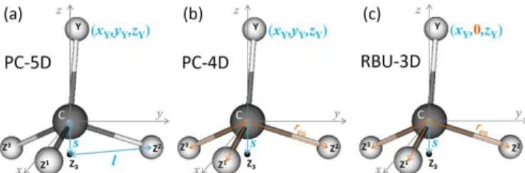
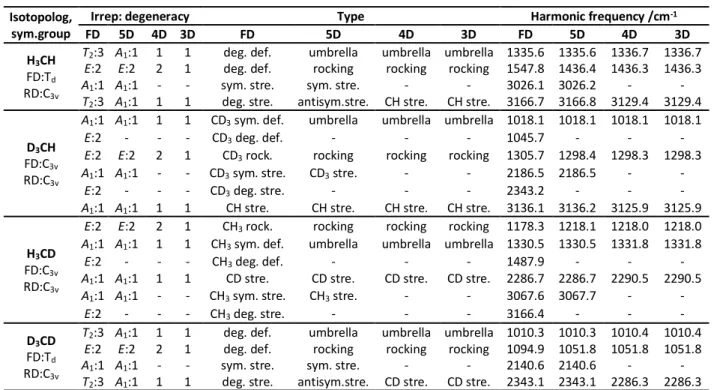
In the following, first we describe the three fundamental coordinate systems used in this work (Section 2.1); then in Section 2.2 we derive the vibrational Lagrangian in body-fixed Cartesian coordinates and then the vibrational Lagrangian and Hamiltonian in internal coordinates (Section 2.3). We discuss the connection of our formulation to the t-vector and s-vector formalisms in both full and reduced-dimensionality (Section 2.4). As applications, normal mode analysis (Section 2.5) and normal mode sampling (NMS, Section 2.6) in internal coordinates and the subsequent transformation of states to laboratory frame are described. In Section 2.7, two methods of RD trajectory integration are presented and compared. Section 2.8 is devoted to the inverse problem, where first the classical state given in laboratory frame is transformed to the internal coordinate system, and the normal coordinate displacements and momenta are calculated, from which the normal mode quantum numbers are determined. The equations presented in Section 2 (apart from Section 2.4) hold not only for reduced- dimensional models but are also applicable in full dimensionality and can also serve as a basis in the derivation of RD quantum Hamiltonians. In Section 3, as a proof of principle, the method is applied to a hierarchy of three RD models of the methane molecule CZ3Y, in each of which the CZ3 group is constrained to maintain C3v symmetry. A complete reaction dynamics study based on this theory has been presented in Ref.

31.

2. Theory

2.1 Frames and Coordinate Systems.

Derivation of the classical vibrational Hamiltonian in internal coordinates starts from the full Lagrangian expressed in Cartesian coordinates in a space-fixed (a.k.a. laboratory) frame:

𝐿(𝐗, 𝐗̇) =^𝟏

𝟐𝐗̇^T𝐌𝐗̇ − 𝐕(𝐗), (1)

where for an 𝑁-atomic system 𝐗 = (𝑋_1𝑥, 𝑋_1𝑦, 𝑋_1𝑧, … , 𝑋_𝑁𝑧)^T and 𝐗̇ are the 3𝑁-component coordinate and corresponding velocity column vectors, respectively, which are composed of the corresponding atomic coordinate 𝐑_𝑖= (𝑋_𝒊𝒙, 𝑋_𝒊𝒚, 𝑋_𝒊𝒛, )^T and velocity 𝐑̇_𝑖 vectors. 𝐌 = diag(𝑚₁, … , 𝑚_𝑁) is the diagonal 3𝑁3𝑁 mass matrix, containing the atomic masses. The classical mechanical state of the system can be given either by the coordinates and the velocities, (𝐗, 𝐗̇) or by the coordinates

and the conjugate momenta,(𝐗, 𝐏_𝑋), the Cartesian momenta being defined as 𝐏_𝑋= 𝐌𝐗̇.

For the description of molecular vibrations, internal coordinates such as valence coordinates (bond lengths, bond and torsion angles etc.) are much more meaningful than Cartesians as the forces acting between atoms are inherently intramolecular, i.e., they do not depend on the position and orientation of the molecule. In addition, the force constants defined in terms of valence coordinates can be rationalized using chemical intuition (for example, they are roughly transferable between molecules)³². Furthermore, the use of internal coordinates is advantageous also when approximations to the Hamiltonian (e.g. quadratic- or quartic-order) are applied as they can describe large amplitude curvilinear motion more effectively than Cartesians.

In general, an internal coordinate is such a function of Cartesian coordinates, whose value is invariant under displacement and rotation of the molecule, thus it is necessarily formulated by using scalar (𝐚𝐛 = 𝐚^𝐓𝐛), and vector (𝐚𝐛) products of atomic Cartesian coordinate vector differences 𝐑_𝑖− 𝐑_𝑗. Consequently, functions of internal coordinates are also internal coordinates. It is worth noting that those internal coordinates that are defined in terms of a cross product (e.g., torsion angles), change sign under mirroring the molecule through a plane (they are pseudoscalars).

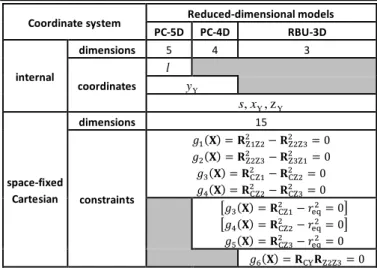
For the description of the vibrating molecule one needs to define 𝑛 independent, otherwise arbitrary internal coordinates 𝐲(𝐗) = (𝑦₁(𝐗), … , 𝑦_𝑛(𝐗))^T in terms of Cartesian coordinates. 𝑛 is less than or may be equal to 𝑓 = 3𝑁 − 6, the number of internal degrees of freedom. If 𝑛 equals 𝑓 then the set of internal coordinates is complete and the model is called full- dimensional. In reduced-dimensional models the set of irredundant internal coordinates is incomplete (𝑛 < 𝑓) and the remaining 𝑓– 𝑛 internal degrees of freedom are constrained by fixing 𝑓– 𝑛 functions 𝑦_𝑛+1(𝐗), … , 𝑦_𝑓(𝐗)at values 𝑦_𝑛+1,0, … , 𝑦_𝑓,0. These constraint functions are generally expressed in terms of the usual valence coordinates. For example, such a function can measure the deviation from some desired symmetry, e.g., it may be the difference of two bond lengths, which is constrained to zero. Variables 𝑦_𝑛+1(𝐗), … , 𝑦_𝑓(𝐗) expressing the constraints are formally internal coordinates, because their values should also be independent of the position and the orientation of the molecule. Note that these constrained variables are not included in vector 𝐲.

In full-dimensional models of vibrating molecules, the kinetic energy in internal coordinates is given with the help of the Wilson 𝐁 matrix evaluated at the instantaneous geometry

19: 𝐁 =^d𝐲

d𝐗 , (2)

The row vectors of the (3𝑁 − 6)3𝑁 dimensional 𝐁 matrix are called vibrational s-vectors ^1,33 (𝐬_𝑖= dy_𝑖/d𝐗). The nonredundant internal coordinates 𝐲 are defined for all values of laboratory coordinates 𝐗, so that the inverse mass matrix

𝐆_y,vib= 𝐁𝐌⁻¹𝐁^T (3)

properly assigns masses to the internal coordinates and the vibrational kinetic energy in internal coordinates written as,

𝐸_kin=1

2𝐩_y^T𝐆_y,vib𝐩_y. (4)

will be exact. However, in reduced-dimensional models (𝑛 < 𝑓), the 𝐗 coordinates are interrelated by the constraints and the 𝐁 matrix defined in (2) with reduced number of rows lacks the information on the corresponding constrained internal coordinates, which is required to disentangle them from the free ones. Consequently, such a reduced-dimensional 𝐁 matrix cannot be used for the construction of the exact reduced- dimensional kinetic energy expression, unless the frozen internal coordinates are orthogonal in some sense to the free ones (see ref. 1 and Section 2.4).

In order to circumvent this problem, we use the inverse transformation, which converts 𝑓 internal coordinates 𝐲 to 3𝑁 lab Cartesian coordinates 𝐗. The inverse function 𝐗(𝐲) and its partial derivatives by definition take into account the constraints because they are evaluated under the condition 𝑦_𝑗(𝐗) = 𝑦_𝑗,0 for 𝑗 = 𝑛 + 1, . . , 𝑓. However, the internal coordinates do not determine the position and orientation of the molecule in the Cartesian system. To locate and orient the molecule one can utilize an intermediate body-fixed frame and an attached Cartesian coordinate system. In this auxiliary body- fixed frame the Cartesian coordinate 3𝑁-vector and the coordinate 3-vector of atom i will be denoted by 𝐱 = (𝑥_1𝑥, 𝑥_1𝑦, 𝑥_1𝑧, … , 𝑥_𝑁𝑧)^T and 𝐫_𝑖= (𝑥_𝒊𝒙, 𝑥_𝒊𝒚, 𝑥_𝒊𝒛, )^T, respectively.

The body-fixed coordinates 𝐱 are connected to the space-fixed frame by an instantaneous translation and rotation, summarized in the function 𝐱(𝐗). The definition of the intermediate frame allows us to derive the Lagrangian in internal coordinates via converting the kinetic and potential energy expressions 1) from space-fixed to body-fixed frame and 2) from body-fixed to internal frame using the inverse transformations 𝐗(𝐱) and 𝐱(𝐲), respectively.

In what follows we proceed on this route in two steps. First we describe the body-fixed frame and its connection to the internal coordinates, 𝐱(𝐲) and then its relationship to the space-fixed Cartesian frame, 𝐗(𝐱) and show how a classical state given in internal coordinates can be transformed into the space-fixed frame.

There are many possible ways of defining a body-fixed Cartesian frame, and it depends on the system which one is the most favorable. One of the simplest possibilities is that one places the origin either at the center of mass of the molecule or at one of the atoms and selects four non-coplanar atoms within the molecule and orthonormalizes three vectors pointing from one of them to the other three to obtain the basis vectors 𝐞_ ( = 𝑥, 𝑦, 𝑧).

The definition of the body-fixed Cartesian coordinates as a function of internal ones is given by a vector-vector function

𝐱 = 𝐱(𝐲), (5)

whose time derivative connects the internal coordinate and the Cartesian velocities:

ARTICLE PCCP

4 | J. Name., 2012, 00, 1-3 This journal is © The Royal Society of Chemistry 20xx

Please do not adjust margins

Please do not adjust margins

𝐱̇ = 𝐂(𝐲)𝐲̇. (6)

The columns of the 3𝑁𝑛 matrix 𝐂(𝐲) = d𝐱/d𝐲 are known as vibrational 𝐭-vectors^1,33,34 (𝐭_𝑖= ∂𝐱/ ∂y_𝑖).

When one knows the 𝐱 coordinates, the Cartesian coordinates of the atoms in the space-fixed frame can be obtained by considering that the body-fixed and space-fixed Cartesian frames can be brought into overlap by a translation and a rotation, i.e., the 𝐫_𝑖 coordinate vectors need to be rotated by matrix 𝐎_frame and shifted by vector 𝐑_frame to get the space- fixed coordinates 𝐑_𝑖:

𝐑_𝑖= 𝐑_frame+ 𝐎_frame𝐫_𝑖. (7)

The atomic velocity 𝐑̇_𝑖 is obtained from that in the body-fixed frame (𝐱̇) by differentiating Eq. (7) with respect to time:

𝐑̇_𝑖= 𝐑̇_frame+ 𝐎̇_frame𝐫_𝑖+ 𝐎_frame𝐫̇_𝑖, (8) where 𝐑̇frame is the velocity of the body-fixed frame with respect to the space-fixed one. To get 𝐎̇frame, one needs to take into account that the body-fixed frame may rotate around its origin with angular velocity _frame. The total time derivative of the rotation matrix 𝐎_frame is then 𝐎̇_frame=_frame× 𝐎_frame, where the cross product of _frame and matrix 𝐎_frame needs to be evaluated column by column. With this, the atomic velocity 𝐑_𝑖 in the space-fixed Cartesian frame is:

𝐑̇_𝒊= 𝐑̇_frame+ (_frame× 𝐎_frame)𝐫_𝑖+ 𝐎_frame𝐫̇_𝑖. (9) Unless special care is taken, the body-fixed frame does not move together with the molecule: its instantaneous linear (𝐑̇_frame) and angular velocities (_frame) differ from those of the molecule in the space-fixed frame. For example, when the body- fixed frame for a vibrating water molecule (H2O) is selected to be centered at the O atom with the 𝑥-axis parallel to H¹H², then the linear velocity of the origin of the frame is not identical to that of the center of mass, and the antisymmetric OH stretch vibration generates angular motion of the molecule (see Fig. 1).

Obviously, the physically correct description of motion requires both the displacements of the atoms of the molecule in the body-fixed frame and translation + rotation of the body- fixed frame in the lab frame. Consequently, the transformation of internal coordinates and momenta to body-fixed frames according to Eqs. (5) and (6) usually generates unphysical (often referred to as spurious ³⁵) translation and rotation.

Figure 1. Schematic drawing of the motion of a water molecule (H¹OH²) in a specific body-fixed frame, which is centered at the O atom with the x-axis parallel to the H¹H² line. Figure (a): the equilibrium geometry with space-fixed displacements (blue arrows) due to antisymmetric stretch vibration. Figure (b) : the distorted molecule and the body- fixed frame aligned according to the new H-H axis. Figure (c) : the distorted molecule when the body-fixed frame is aligned as in Figure (a), showing the corresponding atomic displacements in the body-fixed frame, which result in a clockwise rotated structure whose center of mass (CM) is displaced upward and to the left in the body-fixed frame.

When the focus is on the vibrational motion of a molecule, however, the general procedure is that the motion of the body- fixed frame is disregarded and extra steps are made to eliminate the spurious rotation and translation which would falsify the effective masses assigned to internal coordinates. In the t- vector formalism the cancellation of spurious rotation is achieved by the introduction of rotational coordinates when vibrational energy levels are calculated^1,2.

In classical mechanics, when a vibrational state is generated by normal mode sampling, the molecule can artificially be cleared of these unwanted velocities³⁶. In general, it is desirable to avoid the appearance of the unphysical translational and rotational terms, a novel way of which is proposed in the following sections.

2.2 Vibrational Lagrangian in Body-Fixed Cartesian Coordinates.

To derive the pure vibrational Lagrangian 𝐿_x,vib(𝐱, 𝐱̇) in body- fixed Cartesian coordinates, first the Lagrangian 𝐿_x(𝐱, 𝐱̇) for the non-translating and non-rotating body-fixed frame is obtained.

To achieve this, one substitutes Eqs. (6) and (7) into Eq. (1) and eliminates the rotational and translational motion of the body- fixed frame by setting 𝐑̇_frame= 𝟎 and _frame= 𝟎. Exploiting that matrix 𝐌 is diagonal and matrix 𝐎_frame is unitary, the kinetic energy function in the new coordinates can be transformed into the same form in body-fixed Cartesian coordinates as it was in the lab Cartesian frame, in accordance with the expectations. The form of the potential energy function will also remain the same because it is a function of internal coordinates only, which are defined with dot and cross products (brief common notation: ×̇), that are also left unchanged by 𝐎_frame.

𝐿_𝑥(𝐱, 𝐱̇)=

= 𝐿(𝐗(𝐱), 𝐗̇(𝐱, 𝐱̇); 𝐑̇_{𝐟𝐫𝐚𝐦𝐞}= 𝟎,_frame= 𝟎) =

= ∑^𝟏_𝟐

𝑵

𝒊=𝟏

𝑚_𝑖𝐑̇^T_𝑖𝐑̇_𝑖− 𝑉({(𝐑_𝑗− 𝐑_𝑘) ×̇ (𝐑_𝑙− 𝐑_𝑚)}) =

= ∑^𝟏_𝟐

𝑵

𝒊=𝟏

𝑚_𝑖𝐫̇_𝑖^T 𝐫̇_𝑖− 𝑉({(𝐫_𝑗− 𝐫̇_𝑘) ×̇ (𝐫_𝑙− 𝐫_𝑚)}) =

=^𝟏_𝟐𝐱̇^T𝐌𝐱̇ − 𝑉(𝐱).

(10)

The curly bracket refers to the sets of products involving the atomic indices (j,k,l,m) that are used in the definition of internal coordinates.

We would like to obtain the pure vibrational Lagrangian. For this we need to decompose the kinetic energy into separate vibrational as well as translational and rotational parts. If one introduces mass-scaled coordinates 𝐱̃ = 𝐌^1/2𝐱, the quadratic form of the kinetic energy expressed in the body-fixed Cartesian frame (𝑇_𝑥) reduces to the square of the mass-scaled velocity vector (𝐱̃̇). This form is advantageous, because it allows one to decompose the instantaneous mass-scaled velocity vector into orthogonal translational, rotational and vibrational parts (we show later how). Once these components, 𝐱̃̇_trans, 𝐱̃̇_rot and 𝐱̃̇_vib

are available, the kinetic energy can also be broken down into the corresponding 𝑇_trans, 𝑇_rot and 𝑇_vib terms:

𝑇_x=¹

2(𝐌¹²𝐱̇)^T𝐌¹²𝐱̇ =¹

2𝐱̃̇² =¹

2(𝐱̃̇_trans² + 𝐱̃̇_rot² + 𝐱̃̇_vib² ) =

= 𝑇_trans+ 𝑇_rot+ 𝑇_vib .

(11)

Consequently, the vibrational part can be obtained by eliminating the components of the mass-scaled velocity that correspond to translation and rotation, i.e., projecting the velocities onto the complementary and orthogonal, instantaneous (geometry-dependent) vibrational subspace. If the 3𝑁3𝑁 matrix that performs the desired projection in the space of mass-scaled velocities is denoted by 𝐏_vib(𝐱), the pure vibrational Lagrangian can be formally written as:

𝐿_x,vib(𝐱, 𝐱̇) =¹

2( 𝐏_vib(𝐱)𝐌¹²𝐱̇)^T 𝐏_vib(𝐱)𝐌¹²𝐱̇ − 𝑉(𝐱) . (12) Utilizing the fact that the orthogonal projectors onto the translational and rotational subspaces, 𝐏_trans and 𝐏_rot(𝐱), can be easily found (see below) and their sum is complementary to 𝐏_vib(𝐱), we define 𝐏_vib(𝐱) in terms of them:

𝐏_vib(𝐱) = 𝐄 − 𝐏_trans−𝐏_rot(𝐱), (13) where 𝐄 is the 3𝑁3𝑁 unit matrix. In the following we define the basis vectors of the translational and rotational subspaces and using them, we construct the corresponding projectors.

The translational subspace of mass-scaled displacements and velocities is spanned by the three 3𝑁-component translational basis vectors 𝐮^trans,𝛼 ( = 𝑥, 𝑦, 𝑧):

𝑢_𝑖𝛾^trans,𝛼= ^{∂𝑥̃𝑖𝛾}

∂𝑥CM,𝛼= (√𝑚1𝐞_𝛼

⋮

√𝑚𝑁𝐞_𝛼 )

𝑖𝛾

= √𝑚𝑖(𝐞_𝛼)_𝛾=

√𝑚𝑖𝛿_𝛼𝛾= (𝐌^1/2 𝐭^trans,𝛼)

𝑖𝛾

(14)

𝑢_𝑖𝛾^trans,𝛼 denotes the  ( = x, y, z) component of the mass-scaled displacement of atom i during translation of the whole molecule along axis  (see Fig. 2a-c). 𝛿_𝛼𝛾 is the Kronecker symbol, which is evaluated using 𝑥 = 1, 𝑦 = 2, 𝑧 = 3 assignments to the possible values of its indices  and . The translational basis vectors are related to translational t-vectors (𝐭^trans,𝛼) by mass- scaling. The translational basis vectors only depend on the masses and are independent of the geometry and also of the choice of the origin of the body-fixed frame. Consequently, the translational subspace is the same at all geometries and thus it includes all finite mass-scaled translations of the molecule.

The rotational subspace is spanned by the three 3𝑁- component rotational basis vectors 𝐮^rot,𝛼(𝐱), which describe the relative magnitude of the mass-scaled displacements of atoms due to an infinitesimal rotation of the molecule around the  principal axis (PA) of the instantaneous moment of inertia tensor ( = 1, 2, 3, but not 𝑥, 𝑦, 𝑧). Rotational basis vectors can be calculated from the orthonormal unit vectors of principal axes 𝐞_𝛼^PA (given in the body-fixed frame) and the instantaneous position vectors of atoms 𝛒_𝑖≔ 𝐫_𝑖− 𝐫_CM(𝑖 = 1, … , 𝑁) relative to the center of mass of the molecule, 𝐫_CM:

𝑢_𝑖𝛾^rot,𝛼(𝐱) = ^{∂𝑥̃𝑖𝛾}

∂𝜑_𝛼^PA= (

√𝑚1(𝐞_𝛼^PA× 𝛒₁)

⋮

√𝑚𝑁(𝐞_𝛼^PA× 𝛒_𝑁) )

𝑖𝛾

=

√𝑚𝑖(𝐞_𝛼^PA× 𝛒_𝑖)

𝛾= √𝑚𝑖∑𝜎=𝑥,𝑦,𝑧∑𝜏=𝑥,𝑦,𝑧𝜀_𝛾𝜎𝜏𝑒_𝛼𝜎^PAρ_𝑖𝜏= (𝐌^1/2𝐭^rot,𝛼)_𝑖𝛾.

(15)

𝑢_𝑖𝛾^rot,𝛼characterizes the relative magnitude of the  component ( = 𝑥, 𝑦, 𝑧) of the mass-scaled displacement of atom I when the molecule is rotated infinitesimally around the  (= 1, 2, 3) principal axis (see Fig. 2d-e). The angle of the rotation around 𝐞_𝛼^PA is denoted by 𝜑_𝛼^PA. 𝜀_𝛾𝜎𝜏 is the Levi-Civita tensor which is evaluated using assignments 𝑥 = 1, 𝑦 = 2, 𝑧 = 3 regarding the possible values of its indices , and . The rotational basis vectors are related to rotational t-vectors (𝐭^rot,𝛼) corresponding to rotations around the principal axes by mass-scaling. The rotational basis vectors depend on the geometry. Thus they can be used to describe only infinitesimal mass-scaled displacements of atoms during the rotation of the molecule.

The translational and the rotational basis vectors are orthogonal to each other, and by normalizing them an orthonormal set of translational and rotational basis vectors, 𝐮₀^trans,𝛼 and 𝐮₀^rot,𝛼(𝐱) can be obtained. The proof of orthogonality and the derivation of the norms of the basis vectors are presented in the Appendix.

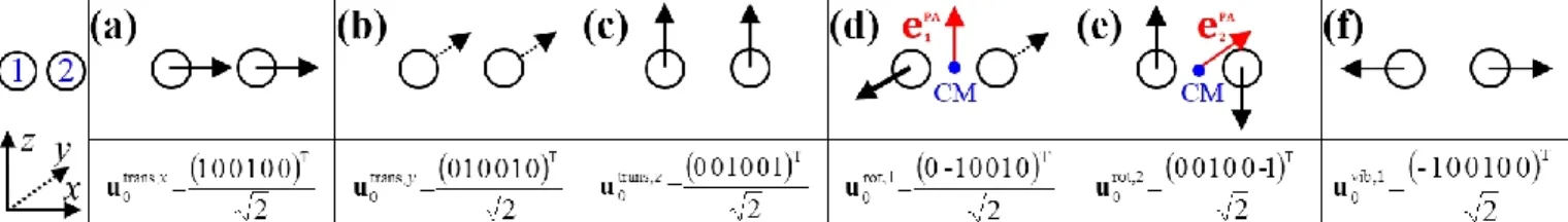
The instantaneous vibrational subspace, which is orthogonal to the translational and rotational subspaces, also depends on the geometry, thus it will span only infinitesimal mass-scaled displacements during the vibration of the molecule. When the shape and the orientation of the molecule do not change during its motion, for example, during the symmetric stretch vibration of CH4 or during the translation of any molecule, the rotational and vibrational subspaces will not change either. A possible orthonormal basis (𝐮₀^vib,𝑖(𝐱_e), 𝑖 = 1, . . , 𝑓 ) of the vibrational subspace at equilibrium geometry (𝐱_𝑒) (is formed by the vibrational normal mode eigenvectors (see Fig. 2f), which are obtained from harmonic vibrational analysis and are mass- scaled by definition. The orthonormal basis vectors of the translational, rotational and vibrational subspaces of a homonuclear diatomic molecule are summarized in Fig. 2. The orthogonal projection matrices 𝐏_trans and 𝐏_rot(𝐱) can be defined as dyadic products (𝐚 ∘ 𝐛 = 𝐚𝐛^T) of the relevant basis vectors:

𝐏_trans= ∑_{𝛼=𝑥,𝑦,𝑧}𝐮₀^trans,𝛼𝐮₀^trans,𝛼,T, (16)

𝐏_rot(𝐱) = ∑³_𝛼=1𝐮₀^rot,𝛼(𝐱) 𝐮₀^rot,𝛼,T(𝐱) . (17) These are the projectors to be used in Eq. (13) to generate the orthogonal projection matrix 𝐏_vib(𝐱) onto the complementary, vibrational subspace. Matrix 𝐏_vib(𝐱), being an orthogonal projector, is idempotent (𝐏_vib² (𝐱) = 𝐏_vib(𝐱)) and symmetric while the mass matrix 𝐌 is diagonal. Consequently, by introducing an effective vibrational mass matrix:

𝐌_vib(𝐱) = 𝐌^1/2𝐏_vib(𝐱)𝐌^1/2, (18)

ARTICLE PCCP

This journal is © The Royal Society of Chemistry 20xx J. Name ., 2013, 00, 1 -3 | 6

Please do not adjust margins Please do not adjust margins Please do not adjust margins

Please do not adjust margins

Figure 2. The three translational (a, b, c), two rotational (d, e) and one vibrational (f) normalized basis vectors of a homonuclear diatomic molecule (H2, O2, etc) at a given orientation.

The Cartesian coordinate system and the indices of atoms are shown in the leftmost panel. In panels (d) and (e), the center of mass (CM) is shown in blue, and the unit vectors along the principal axes are shown in red.

which is geometry dependent and dense as opposed to matrix 𝐌, the Lagrangian in Eq. (12) can be rewritten in the form:

𝐿_x,vib(𝐱, 𝐱̇) =¹

2𝐱̇^T𝐌_vib(𝐱)𝐱̇ − 𝑉(𝐱). (19) Matrix 𝐌_vib(𝐱)is singular, since it assigns non-zero masses only to the motion within the vibrational subspace, which has fewer dimensions than 3𝑁. Momenta 𝐩_x,vib canonically conjugate to coordinates 𝐱 are obtained by differentiating the Lagrangian:

𝐩x,vib=^d𝐿x,vib_d𝐱̇^{(𝐱,𝐱̇)}= 𝐌vib(𝐱)𝐱̇. (20) While the velocity vector may describe translation and rotation in addition to vibration of the molecule in the body- fixed frame, the momentum vector 𝐩_x,vib describes only vibrations, because it is obtained by the singular mass matrix 𝐌_vib(𝐱). Thus, the Legendre transformation to obtain the corresponding Hamiltonian cannot be done in the regular way.

We note that the present derivations are similar to the projection method proposed by Miller et al..³⁷ Szalay³⁸ for the approximate decomposition of the kinetic energy in the Eckart frame. The difference is that we apply the exact decomposition of the instantaneous kinetic energy.

2.3 Vibrational Hamiltonian in Internal Coordinates

The vibrational Lagrangian in internal coordinates 𝐲 and velocities 𝐲̇ can be obtained from Eq. (19) using the transformations in Eqs. (5) and (6):

𝐿_y,vib(𝐲, 𝐲̇) =¹

2(𝐂(𝐲)𝐲̇)^T𝐌_vib(𝐱(𝐲)) 𝐂(𝐲)𝐲̇ − 𝑉(𝐱(𝐲)) =

=¹

2𝐲̇^T𝐌_y,vib(𝐲)𝐲̇ − 𝑉_𝑦(𝐲).

(21)

Here we introduced the potential energy 𝑉_𝑦(𝐲) = 𝑉(𝐱(𝐲)) as well as the 𝑛𝑛 vibrational mass matrix as functions of internal coordinates 𝐲:

𝐌_y,vib(𝐲) = 𝐂^T(𝐲)𝐌^1/2𝐏_vib(𝐱(𝐲))𝐌^1/2 𝐂(𝐲). (22) At this point, it becomes obvious that by projecting onto the vibrational subspace, we cancel the spurious translation and rotation in the body-fixed frame and the masses corresponding to them will not contaminate the mass matrix assigned to the internal coordinates, which would unphysically increase the matrix elements. Without the projection, for example, harmonic vibrational analysis would give incorrect, reduced frequencies for some of the normal modes.

Eq. (22) applies as it is when 𝑛 = 𝑓. Its form implies that in reduced-dimensional models the reduced-dimensional 𝐌_y,vib(𝐲) matrix can be obtained from the full-dimensional 𝐌_y,vib by simply deleting the rows and columns corresponding to the constrained internal coordinates.

Momenta canonically conjugate to the internal coordinates are obtained as:

𝐩_𝑦=^{∂𝐿y,vib(𝐲,𝐲̇)}

∂𝐲̇ = 𝐌_y,vib(𝐲)𝐲̇, (23)

and the velocity 𝐲̇ as a function of 𝐲 and 𝐩_𝑦 will be

𝐲̇ = 𝐌_y,vib⁻¹ (𝐲)𝐩_𝑦= 𝐆_y,vib(𝐲)𝐩_𝑦. (24) Here, the 𝑛𝑛 dimensional 𝐆_y,vib(𝐲) matrix is the inverse of the non-singular 𝐌_y,vib(𝐲) matrix. Applying Legendre transformation to the Lagrangian, one can obtain the vibrational Hamiltonian in internal coordinates:

𝐻_y,vib(𝐲, 𝐩_𝑦) = 𝐩_𝑦^T𝐲̇(𝐲, 𝐩_𝑦) − 𝐿_y,vib(𝐲, 𝐲̇(𝐲, 𝐩_𝑦)) =

=¹

2𝐩_𝑦^T𝐆_y,vib(𝐲)𝐩_𝑦+ 𝑉_𝑦(𝐲).

(25)

This form is correct in any nonredundant set of internal coordinates, be it reduced (𝑛 < 𝑓) or complete (𝑛 = 𝑓).

2.4 Connection with the t-vector and the s-vector Formalisms In the previous two sections we derived the vibrational kinetic energy in internal coordinates by introducing the body- fixed frame 𝐱 and using the inverses of the arbitrarily defined 𝐱(𝐗) and 𝐲(𝐱) transformations. In this section we show the relationship of our method to those that are generally used for this purpose in the literature, one those based on the 𝐗 → 𝐲 transformation ^1,33,39 (s-vector formalism) as well as on the 𝐲 → 𝐱 transformation ^1,40 (t-vector formalism).

The s-vector formalism provides the exact vibrational Hamiltonian for the full-dimensional vibrational problem. To derive the reduced-dimensional kinetic energy and the mass matrices using the 𝐗 → 𝐲 transformation, it is necessary to extend the set of variables to a full set of internal variables and first construct the full-dimensional 𝐆_𝑦,vib (see Eq. (3)), then calculate the full-dimensional 𝐌_𝑦,vib by inversion. Then columns and rows corresponding to the constrained variables are omitted from it as it is done in the case of the method proposed in the present paper, and finally the reduced- dimensional 𝐆_𝑦,vib matrix is calculated by inversion.

x

)

vib(

y , y

M

The t-vector formalism requires the definition of a body- fixed frame (e.g., Eckart frame⁴¹), which is rarely the absolute co-rotating frame. To compensate for the arising spurious rotation during the change of internal coordinates of the molecule, rotational coordinates need to be introduced and a rovibrational Hamiltonian has to be constructed to make possible the exact description of the vibrational problem. The reduced-dimensional Hamiltonian is directly obtained by using only those vibrational t-vectors which belong to non- constrained internal variables.

The method presented in this work is analogous to the t- vector formalism also in the sense that both are based on the d𝐱/d𝐲 derivatives and allow the direct construction of a reduced-dimensional Hamiltonian. However, instead of introducing rotational variables, our method exploits the orthogonality of the mass-scaled translational and (instantaneous) rotational basis vectors (3𝑁-component) to vibrational ones so that rotation and translation are exactly removed. This approach provides a pure vibrational kinetic energy expression equivalent with the one provided with the s- vector formalism.

It can be shown that the inverse mass matrix 𝐆_𝑦,vib in the s- vector formalism (Eq. (3)) is the inverse of the 𝐌_𝑦,vib mass matrix in Eq. (22).and that this does not hold for the reduced- dimensional case as the pure-vibrational infinitesimal mass- scaled Cartesian displacement vectors corresponding to the various internal coordinates are not orthogonal to each other in general. This also implies that the s-vector formalism in full internal dimensionality is in fact a reduced-dimensional approximation, because it considers only vibrations and translational and rotational coordinates are simply omitted.

This raises the question how it can be exact for vibrations. The reason for this is the inherent orthogonality of vibrations to rotations and translations in mass-scaled infinitesimal displacement space.

2.5 Normal Mode Analysis in Internal Coordinates

During normal mode analysis the vibration of the molecule is approximately decomposed into independent harmonic oscillators using the harmonic approximation to the kinetic and potential energy expressions. The harmonic approximation to the Lagrangian in internal coordinates in the neighborhood of a stationary point𝐲₀ can be obtained by replacing the 𝐌_{𝑦 ,vib}(𝐲) matrix function with its value at 𝐲₀, 𝐌_y,vib,0= 𝐌_y,vib(𝐲₀), approximating the potential energy to second order around 𝐲₀, and setting its zero level to that at geometry 𝐲₀:

𝐿^harm_y,vib(𝐲, 𝐲̇) =¹

2𝐲̇^T𝐌_y,vib,0𝐲̇ −¹

2(𝐲 − 𝐲₀)^T𝐅_y,0(𝐲 − 𝐲₀). (26) Here 𝐅_y,0= 𝑉_y^″(𝐲₀) is the force constant matrix. This generally proves to be a good approximation to the Lagrangian at low energies in semi-rigid molecules, where no internal rotations or other large amplitude motion can take place.

From here on one can follow the standard procedure of normal mode analysis. After introducing mass-scaled vectors of deformation 𝐲̃ = 𝐌_y,vib,0^1/2 (𝐲 − 𝐲₀) and velocity 𝐲̃̇ = 𝐌_y,vib,0^1/2 𝐲̇

and the 𝐅̃_y,0= 𝐆_y,vib,0^1/2 𝐅_y,0𝐆_y,vib,0^1/2 mass-scaled force constant

matrix (where 𝐆_y,vib,0= 𝐌_y,vib,0⁻¹ ) one solves its 𝐅̃_y,0𝐔=𝐔

eigenproblem. Matrix 𝐅̃_y,0 is symmetric, thus all 𝑛 eigenvalues

_𝑖 (in matrix = diag(₁, . . ,_𝑛)) are real and the eigenvectors (i.e. columns of 𝐔) can be chosen to be orthonormal. If 𝐲₀ is a potential minimum, all eigenvalues are positive, whereas for a 𝑘^th-order saddle point 𝑘 of them are negative. The vector of normal-mode deformation coordinates 𝐐 = (𝑄₁, . . , 𝑄_𝑛)^T and the canonically conjugate momentum vector 𝐏 = (𝑃₁, . . , 𝑃_𝑛)^T (in fact, the normal-mode velocity vector 𝐐̇) are defined as:

𝐐 = 𝐔^T𝐲̃ = 𝐔^T𝐌_y,vib,0^1/2 (𝐲 − 𝐲₀), (27)

𝐏 = 𝐐̇ = 𝐔^T𝐲̃̇ = 𝐔^T𝐌_y,vib,0^1/2 𝐲̇. (28) In normal coordinates both the Lagrangian and the Hamiltonian (i.e. energy) decompose into sums of 𝑛 harmonic oscillator (HO) terms:

𝐻_harm,𝑖^1D (𝑄_𝑖, 𝑃_𝑖) = 𝐸_harm,𝑖^1D =¹

2𝑃_𝑖²+¹

2ω_𝑖² 𝑄_𝑖²=

=¹

2𝑄̇_𝑖²+¹

2ω_𝑖² 𝑄_𝑖².

(29)

The normal mode frequencies can be obtained as 𝜔_𝑖= 𝜆_𝑖^1/2. 2.6 Normal Mode Sampling

The purpose of normal mode sampling is the generation of a set of classical states corresponding to a preselected vibrational state of a reactant molecule that will serve as initial conditions for collision or intramolecular trajectories. In QCT calculations, the initial states of molecules are usually generated by assuming that vibration and rotation are separable and the vibrations are well described by the normal mode approximation. The procedure for normal mode sampling is well known for full- dimensional models, but without the proper RD normal mode analysis, it cannot be used in reduced dimensionality. In normal mode sampling it is assumed that the vibrating molecule can be well approximated as a set of independent normal oscillators with 𝑛 distinct quantum numbers 𝑣₁, … , 𝑣_𝑛 (𝑛 constants of motion). In quasiclassical quantization, normal coordinate and momentum amplitudes (𝑄_𝑖,max, 𝑃_𝑖,max= 𝑄̇_𝑖,max) of each normal mode oscillator are set so that the energy of the oscillator (𝐸_harm,𝑖^1D ) matches that of the corresponding quantum harmonic oscillator in a given 𝑣_𝑖 quantum state:

𝐸_harm,𝑖^1D =¹

2ω_𝑖² 𝑄 _𝑖,max² =¹

2𝑃_𝑖,max² =¹

2𝑄̇_𝑖,max² =

= ℏω _𝑖(𝑣_𝑖+¹

2).

(30)

For the generation of classical states (𝐐, 𝐏), a random initial phase _𝑖,0 is selected from a uniform distribution in the [0,2) interval for each vibrational mode, and then the normal mode coordinate and velocity of normal oscillator 𝑖 can be calculated according to:

𝑄_𝑖= 𝑄_𝑖,maxcosφ_𝑖,0, (31)

𝑃_𝑖= 𝑄̇_𝑖= −𝑄̇_𝑖,maxsinφ_𝑖,0. (32)

ARTICLE PCCP

8 | J. Name., 2012, 00, 1-3 This journal is © The Royal Society of Chemistry 20xx

Please do not adjust margins

Please do not adjust margins

The corresponding classical state (𝐲, 𝐲̇) in internal coordinates can be obtained by inverting Eqs. (27) and (28):

𝐲 = 𝐲0+ 𝐆_y,vib,0^1/2 𝐔𝐐, (33)

𝐲̇ = 𝐆_y,vib,0^1/2 𝐔𝐏 = 𝐆_y,vib,0^1/2 𝐔𝐐̇. (34) The resulting classical state (𝐲, 𝐲̇) is the appropriate initial state if one intends to follow the time evolution of the system using the Euler-Lagrange or Newton equations of motion. If one would like to describe the same dynamics in the more convenient Hamiltonian formalism (see Section 2.7.1), then the initial state should be expressed in internal coordinates and the conjugate momenta (𝐲, 𝐩_y), where the momenta are obtained from Eq. (23) with the mass matrix 𝐌_y,vib(𝐲) calculated at the instantaneous geometry 𝐲.

When the trajectory integration is to be performed in Cartesian coordinates, the state (𝐲, 𝐲̇) needs to be transformed to the body-fixed Cartesian frame and one should ensure that the unphysical translation and rotation generated during transformations in Eqs. (5) and (6) are removed. To obtain the pure vibrational classical state (𝐱, 𝐩_𝑥,vib), the body-fixed Cartesian coordinates 𝐱 are calculated from 𝐲 using Eq. (5); the corresponding Cartesian momenta describing vibration only are found by transforming 𝐲̇ to 𝐱̇ with matrix 𝐂(𝐲) and finally to 𝐩_𝑥,vib with matrix 𝐌_vib(𝐱) using Eqs. (6) and (20), respectively:

𝐩_𝑥,vib= 𝐌_vib(𝐱)𝐱̇ = 𝐌_vib(𝐱(𝐲))𝐂(𝐲)𝐲̇. (35) The point here is that the geometry-dependent mass matrix 𝐌_vib(𝐱), which assigns mass only to vibrations, guarantees that the resulting classical states (𝐱, 𝐩_𝑥,vib) will have zero center-of-mass momentum and angular momentum. The coordinate and velocity conversion equations also ensure that Cartesian coordinates 𝐱, velocities 𝐱̇ and momenta 𝐩_𝑥,vib fulfill the equations of geometrical constraints (𝑦_𝑛+1(𝐱) = 𝑦_𝑛+1,0, … , 𝑦_𝑓(𝐱) = 𝑦_𝑓,0) and their time derivatives (see Section 2.7.2).

The ensemble of classical states (𝐱, 𝐩_𝑥,vib) in Cartesian coordinates, which corresponds to the pre-selected vibrational quantum state of the reduced-dimensional model of the reactant molecule is generated by carrying out the sampling procedure many times with different random phases in Eqs.

(31) and (32). It should be noted that the ensemble obtained this way is not monoenergetic. In QCT calculations the nonrotating molecules are randomly oriented before collision.

If a rovibrational state is to be generated, then the molecule’s angular momentum is also set to that of the desired quantum state. The obtained classical states are in laboratory Cartesian frame and thereby they can be used in the definition of initial conditions of the molecule (𝐗, 𝐏_𝑋), for QCT calculations

The standard method to prepare monoenergetic ro- vibrating ensembles by iterative rescaling of deformations and momenta and angular momentum vector adjustment after normal mode sampling has been proposed by Hase and coworkers ⁴². That method can be generalized to reduced- dimensional models. What remains the same is that the scaling

factor is determined in the lab frame. The important difference is that in the full-dimensional model the scaling factor can be applied to scale the lab-frame deformations and momenta. In RD models the rescaling step needs to be performed in internal coordinates, because otherwise it would violate the constraints.

It should be noted that the ensembles generated this way are not stationary when allowed to evolve on the real, anharmonic PES²¹. Monoenergetic, stationary and accurately quantized ensembles of classical states representing a rovibrational quantum state can be generated by applying the adiabatic principle of classical mechanics. A generalized version of the adiabatic switching method, which accurately includes anharmonicity and coupling of vibrations, has recently been shown to perform well for polyatomic molecules. ⁴³ The method has also been extended to generate ensembles corresponding to rovibrational quantum states.

2.7 Dynamics in Reduced Dimensionality.

In reduced-dimensional classical trajectory calculations the equations of motion for the intramolecular motion of molecules have to guarantee the fulfillment of the constraints prescribed by the model. In the following, we discuss two choices: the application of equations of motion in internal coordinates and the integration of the equations of motion in lab Cartesian frame, supplemented by constraint forces. Integration in internal coordinates is more appropriate for the description of a vibrating molecule, whereas the equations presented for integration in 3𝑁 Cartesians are equally applicable both to pure bound motion and to scattering problems.

2.7.1 Equations of Motion in Internal Coordinates. Hamiltonian equations of the pure vibrational motion in internal coordinates can be derived from the Hamiltonian in Eq. (25).

𝐩̇_y= −^{𝜕𝐻y,vib(𝐲,𝐩y)}

𝜕𝐲 = −¹

2𝐩_y^T𝐆^′_y,vib(𝐲)𝐩_y− 𝑉_y′(𝐲) , (36) 𝐲̇ = −^{𝜕𝐻y,vib(𝐲,𝐩y)}

𝜕𝐩_y = 𝐆_y,vib(𝐲)𝐩_y. (37)

Rank-3 tensor 𝐆^′_y,vib(𝐲) and vector 𝑉_y′(𝐲) are the coordinate derivatives of the inverse mass matrix 𝐆_y,vib(𝐲) and the potential energy 𝑉_𝑦(𝐲). The initial conditions of the motion can be obtained via Eqs. (33) and (34) and formula 𝐩_y= 𝐌_y,vib(𝐲)𝐲̇.

When vibrational dynamics are simulated, internal to body- fixed frame transformation and projection onto the vibrational subspace have to be performed several times at every integration step for the evaluation of 𝐆_y,vib(𝐲), 𝐆′_y,vib(𝐲) and 𝑉_y′(𝐲) (see Eqs. (5), (6), (22) and (24)). The generally involved calculation of the rank-3 𝐆′_y,vib(𝐲) derivative tensor can be sped up by using some analytical transformations (see ESI). A more serious drawback of using internal coordinates is that they may become indeterminate and in that neighborhood they change very steeply. At these points the coordinate transformation in Eq. (5) or its inverse has singularities, which can cause significant numerical errors during the solution of the equations of motion. For example, such a singularity arises for 3D polar coordinates (𝑟,,) at small ( 0) and large ( 180) polar angles where  may change very quickly during

dynamics. With careful selection of the body-fixed frame and the set of internal coordinates one can achieve that the singularities of the transformation equations (Eqs. (5) and (6)) will be at highly deformed geometries which are not sampled by normal mode state preparation and not visited during the vibration of the molecule. It is important to emphasize that Eqs.

(36) and (37) describe the vibration of non-rotating molecules only.

2.7.2 Equations of Motion with Constraints in Space-Fixed Cartesian Coordinates. During the internal motion of floppy molecules, as well as in loose clusters and chemical reactions, where bonds get broken and formed, highly-deformed geometries are visited and the moieties of reactant molecules can have arbitrary orientation with respect to each other. For such systems, it is preferable to simulate the reduced- dimensional dynamics by integrating the equations of motion in the full set of 3𝑁 lab Cartesian coordinates (𝐗) and enforcing the restrictions in the internal degrees of freedom by constraint forces. To derive constraint forces, we introduce functions 𝑔_𝑖(𝐗) (𝑖 = 1, … , 𝑓– 𝑛) as the deviations of functions 𝑦_𝑛+𝑖(𝐗) from their corresponding frozen values 𝑦_𝑛+𝑖,0. The equations of constraints are obtained by equating the 𝑔_𝑖(𝐗) functions to zero.

𝑔_𝑖(𝐗) ≔ 𝑦_𝑛+𝑖(𝐗) − 𝑦_𝑛+𝑖,0= 0 𝑖 = 1, … , 𝑓– 𝑛 (38) These constraints are holonomic as they depend only on the position coordinates (but not on their time derivatives) and are scleronomic as they do not depend on time explicitly. They are expected to be fulfilled all along a trajectory, implying that their time derivatives must also be zero:

𝑔̇_𝑖(𝐗, 𝐗̇) = ∇^T𝑔_𝑖𝐗̇ = ∇^T𝑔_𝑖𝐌⁻¹𝐏_X= 0 𝑖 = 1, … , 𝑓– 𝑛, (39) which serve as constraint equations for the velocities 𝐗̇ and momenta 𝐏_X. Consequently, a mechanical state, which is fully characterized either by (𝐗, 𝐗̇) or (𝐗, 𝐏_X), should fulfill Eqs. (27) and (28) simultaneously. The 3𝑁-component constraint force arising from constraint 𝑖 in Eq. (39) is necessarily parallel to gradient ∇𝑔_𝑖, because it confines the allowed motion (velocity 𝐗̇) to a (3𝑁 − 1)-dimensional surface orthogonal to ∇𝑔_𝑖. Consequently, each constraint force 𝐅_𝑖^constr is expressed as being proportional to ∇𝑔_𝑖 which, multiplied by Lagrange multipliers 𝜆_𝑖 (𝑖 = 1, . . , 𝑓– 𝑛) are added to Hamilton’s equations for momenta, supplementing there the potential forces:

𝐏̇_X= −∇𝑉 + ∑ 𝐅_𝑖^constr

𝑓−𝑛

𝑖=1

= −∇𝑉 + ∑ 𝜆_𝑖∇𝑔_𝑖

𝑓−𝑛

𝑖=1

. (40)

The Hamiltonian equations of motion for the coordinates remain the same (𝐗̇ = 𝐌⁻¹𝐏_X) since the constraints in Eq. (38) are holonomic. The Lagrange multipliers need to be calculated at every time step of trajectory integration via a set of linear equations. An excellent description of how the Lagrange multipliers are determined in practice can be found in Refs. 3, 4 and 20. For completeness, the equations with the present notations are summarized in the ESI.

2.7.3 Comparison of the Computational Aspects of the Two Descriptions. Usually the most expensive part of trajectory simulations is the evaluation of potential gradients. If no analytical gradients of the potential energy are available, then they need to be evaluated numerically with finite difference formulae, whose computational cost scales linearly with the number of gradient components. When nonredundant internal coordinates are used, some computational savings come from the reduced number (𝑓 < 3𝑁 − 6) of gradient components in the 𝑉_y′(𝐲) potential gradient compared to the full-dimensional Cartesian problem (3𝑁). On the other hand, simulation of the dynamics in irredundant internal coordinates requires repeated evaluation of rank-3 tensor 𝐆′_y,vib(𝐲), which can be expensive unless analytical first and second derivatives (matrices 𝐂(𝐲) and 𝐂′(𝐲)) of the coordinate transformation 𝐱(𝐲) are available.

Analytical derivation of matrix 𝐂 can be complicated and requires non-negligible human effort even when computer algebra packages are employed, and even when the derivatives are available, their evaluation may require numerous algebraic operations.

In the alternative method, integration of the equations of motion in Cartesian coordinates under the control of constraints, at least 6 more potential gradient components need to be evaluated; in addition, the constraint forces need to be determined. Yet, the application of Cartesian coordinates together with constraints can be overall cheaper than using internal coordinates, especially when analytic first derivatives of the PES, and first and second analytic derivatives of the constraints are available.

An additional aspect is the accuracy to which the constraints prescribed by the reduced-dimensional model are fulfilled.

Integrating in internal coordinates automatically satisfies these constraints. On the other hand, when full-dimensional Cartesian coordinates are used, the constraints are enforced numerically, so that their fulfillment (Eqs. (38) and (39)) depends on the accuracy of the numerical procedure. Accordingly, in long simulations it is desirable to check regularly how well the constraints are met. If any of them is violated significantly, fulfillment of them can be reestablished by minimizing to zero the sum of the properly scaled squares of the left hand sides of Eqs. (38) and (39).

2.8 Assignment of Normal Mode Quantum Numbers to Reduced- Dimensional Classical States.

Solution of the inverse problem, determination of normal mode quantum numbers corresponding to a reduced- dimensional classical state of the molecule is needed when product-state resolved properties are calculated for bimolecular reactions or when the classical evolution of vibrationally excited states of molecules is of interest.

Depending on which of the two sets of Hamiltonian equations of motion (Section 2.7) were used for trajectory integration, the classical state of the system is provided either in nonredundant internal coordinates and momenta (𝐲, 𝐩_𝑦) or in space-fixed Cartesian coordinates and momenta (𝐗, 𝐏_𝑋) fulfilling constraints in Eqs. (38) and (39).